Run this strategy
Copy the prompt to reproduce the evidence above with the article’s data, assumptions, and risk checks.
Tell your AI:
Set up FinLab and rerun the seven lazy portfolios against QQQ. Please read: https://finlab.finance/en/setup?relatedUrl=/en/blog/lazy-portfolio-backtest
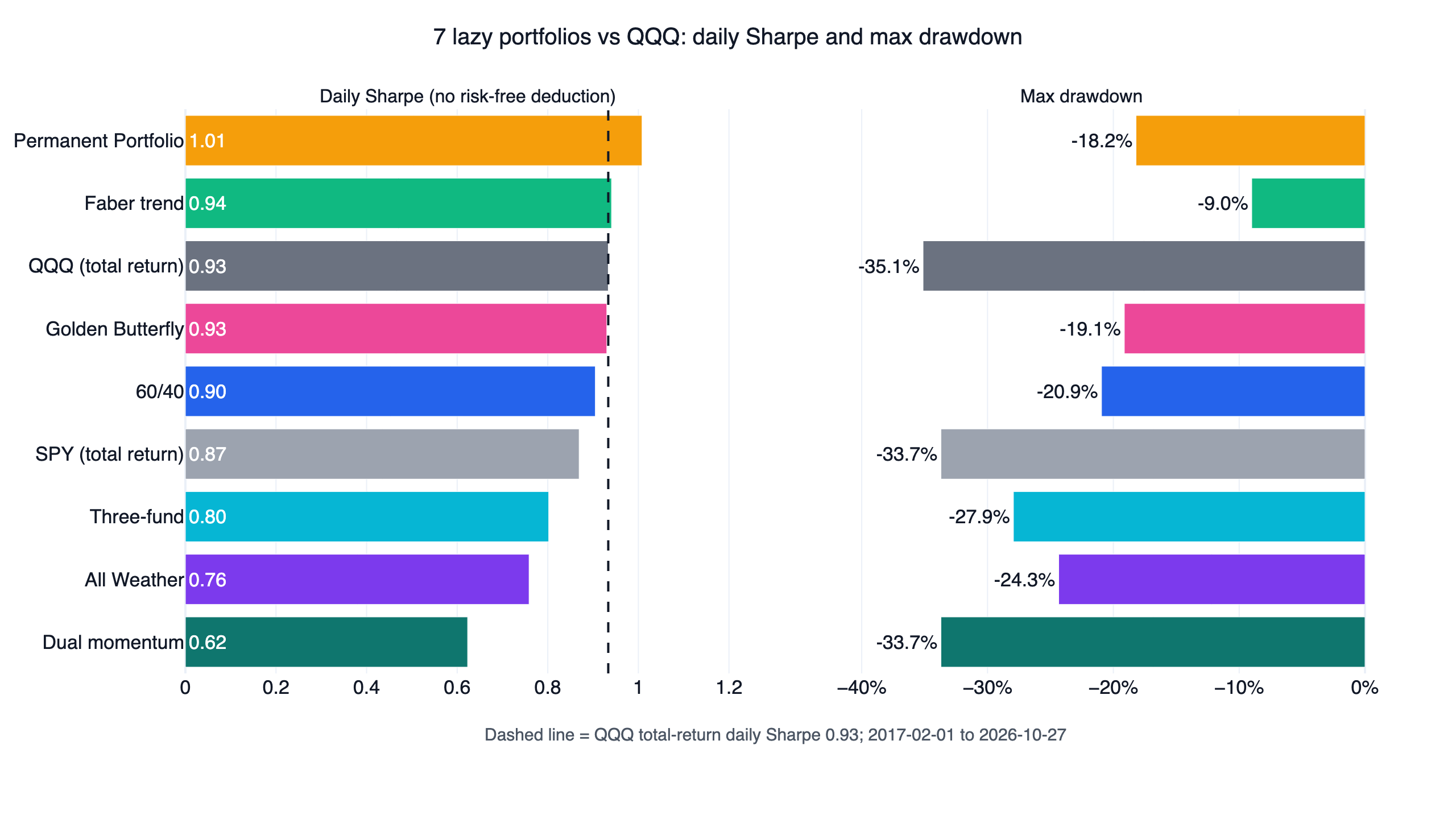
We backtested the seven most quoted lazy portfolios on US ETFs from February 2017 to October 2026: 60/40, the Bogleheads three-fund portfolio, All Weather, the Permanent Portfolio, the Golden Butterfly, and two rules-based allocations, Faber's trend-following model and Antonacci's dual momentum. Every one of them had a shallower maximum drawdown than QQQ's -35.1%, and Faber's was only -9.0%. None of them beat QQQ on risk-adjusted return across all three of our robustness checks. The two closest each failed one check. The Permanent Portfolio posted a full-period daily Sharpe of 1.01 against 0.93 for QQQ and won both halves of the window, but cutting its stock weight from 25% to 15% turned three of its nine parameter settings into losers. Faber's model won eight of nine settings, yet lost the first half (2017 to 2021) with 1.12 against QQQ's 1.20.
The seven portfolios at a glance
| Portfolio (source) | ETFs and weights | Daily Sharpe | CAGR | Max drawdown | Settings beating QQQ | First / second half Sharpe |
|---|---|---|---|---|---|---|
| Permanent Portfolio (Browne) | VTI, TLT, GLD, BIL at 25% each | 1.01 | 7.7% | -18.2% | 6/9 | 1.38 / 0.75 |
| Faber trend (Faber 2007) | SPY, EFA, IEF, VNQ, DBC at 20% each; below the 10-month average, that slice goes to BIL | 0.94 | 6.3% | -9.0% | 8/9 | 1.12 / 0.76 |
| Golden Butterfly (Portfolio Charts) | VTI, VBR, TLT, SHY, GLD at 20% each | 0.93 | 8.4% | -19.1% | 0/9 | 1.22 / 0.70 |
| 60/40 | SPY 60%, AGG 40% | 0.90 | 10.0% | -20.9% | 0/9 | 1.12 / 0.69 |
| Three-fund (Bogleheads) | VTI 56%, VXUS 24%, BND 20% | 0.80 | 10.9% | -27.9% | 0/9 | 0.92 / 0.68 |
| All Weather (simplified Dalio) | VTI 30%, TLT 40%, IEF 15%, GLD 7.5%, DBC 7.5% | 0.76 | 6.5% | -24.3% | 0/9 | 1.41 / 0.29 |
| Dual momentum (Antonacci 2014) | One of SPY, VXUS or AGG each month | 0.62 | 9.5% | -33.7% | 0/9 | 0.62 / 0.63 |
| QQQ (total return) | Buy and hold | 0.93 | 20.5% | -35.1% | Benchmark | 1.20 / 0.67 |
| SPY (total return) | Buy and hold | 0.87 | 15.1% | -33.7% | Reference | 0.97 / 0.75 |
Every portfolio runs from 2017-02-01 to 2026-10-27; QQQ and SPY are buy-and-hold with dividends reinvested over the same trading days. The halves split on 2021-12-10. The Golden Butterfly's Sharpe is 0.930 against QQQ's 0.934, so the two look tied after rounding but the portfolio loses; Faber's 0.941 is a narrow win.
How a portfolio had to pass
"Beats QQQ" has one meaning here: a higher daily Sharpe ratio than buying and holding QQQ with dividends reinvested, over exactly the same trading days. Daily Sharpe is the mean daily return divided by its standard deviation, times the square root of 252, with no risk-free rate deducted. A portfolio counts as working only if it clears all three checks:
- Neighbouring parameters. Each portfolio has two main parameters; we test the original value and one step either side of each, nine settings in total, and at least seven of the nine (a 70% threshold, rounded up) must beat QQQ. For 60/40, All Weather, the Permanent Portfolio and the Golden Butterfly the parameters are the stock weight (original plus or minus 10 percentage points, other assets scaled pro rata) and the rebalancing frequency (monthly, quarterly, yearly). For the three-fund portfolio they are the bond weight (10%, 20%, 30%) and the international share of the stock sleeve (20%, 30%, 40%). Faber's are the moving-average length (8, 10, 12 months) and a band (price must be above 99%, 100% or 101% of the average to hold). Dual momentum's are the relative and absolute lookbacks (9, 12, 15 months each); the five settings that use a 15-month lookback cannot start until the end of April 2017, so they run from 2017-05-01 and are compared with QQQ over those same days (daily Sharpe 0.90).
- Both halves. Split the window at its midpoint; the original setting must beat QQQ in each half on its own, so one strong stretch cannot carry the result.
- Full period, with default costs. Over the whole window, under finlab's default US costs in
sim()(no commission and no tax, matching mainstream zero-commission brokers), the portfolio must beat QQQ. We also ran a 0.1%-per-side stress test to see how much the two rules-based portfolios, which trade more, would give up.
Zero of the seven cleared all three. Faber edges past QQQ at default costs (0.941 against 0.934), but at 0.1% per side it drops to 0.88 and loses even the full period. Check by check:
| Portfolio | Neighbouring parameters | Both halves | Full period at default costs | 0.1% per side stress |
|---|---|---|---|---|
| Permanent Portfolio | ✗ 6/9 | ✓ | ✓ 1.01 | 1.01 |
| Faber trend | ✓ 8/9 | ✗ first half 1.12 | ✓ 0.941 | 0.88 (CAGR 5.9%) |
| Golden Butterfly | ✗ 0/9 | ✓ | ✗ 0.930 | 0.93 |
| 60/40 | ✗ 0/9 | ✗ first half 1.12 | ✗ 0.90 | 0.90 |
| Three-fund | ✗ 0/9 | ✗ first half 0.92 | ✗ 0.80 | 0.80 |
| All Weather | ✗ 0/9 | ✗ second half 0.29 | ✗ 0.76 | 0.76 |
| Dual momentum | ✗ 0/9 | ✗ both halves | ✗ 0.62 | 0.60 (CAGR 9.0%) |
The seven portfolios and how each was built
All prices are finlab's us_fund_price:adj_close, closes adjusted for reinvested distributions. Fixed-weight portfolios rebalance back to target at the last close of each quarter; the two rules-based portfolios read their signal at the last close of each month, and sim() trades at the next day's close.
- 60/40. Sixty percent stocks and forty percent bonds is the textbook balanced allocation used by balanced funds, built on the idea that stocks and bonds have low correlation, so the mix is much less volatile than stocks alone. We use SPY (S&P 500) and AGG (US aggregate bonds).
- Bogleheads three-fund portfolio. The Bogleheads community distilled John Bogle's indexing case into three total-market funds: US stocks, international stocks and US bonds, as described on the Bogleheads wiki. There is no official mix; we use 80% stocks and 20% bonds with 30% of the stock sleeve international, which is VTI 56%, VXUS 24%, BND 20%.
- All Weather. Ray Dalio's Bridgewater sizes positions by risk ("risk parity") so that some asset holds up whether growth or inflation rises or falls. The retail version most people know is the simplified mix Tony Robbins published in Money: Master the Game (2014): 30% stocks, 40% long-term Treasuries, 15% intermediate Treasuries, 7.5% gold and 7.5% commodities. Institutional risk parity levers up the low-risk assets; Asness, Frazzini & Pedersen (2012) argue that because most investors cannot or will not use leverage, low-risk assets earn higher risk-adjusted returns, and risk parity captures that gap by holding them with leverage. We test the unlevered retail version.
- Permanent Portfolio. Harry Browne proposed it in the 1980s and laid it out in Fail-Safe Investing (1999): 25% each in stocks, long-term Treasuries, gold and cash, one asset for each of prosperity, deflation, inflation and recession. We use VTI, TLT, GLD and BIL (1-3 month T-bills).
- Golden Butterfly. Tyler of the Portfolio Charts site reworked the Permanent Portfolio: cash is replaced entirely by short-term Treasuries (SHY), stocks rise from 25% to 40% (20% each in total-market VTI and small-cap value VBR), and long Treasuries (TLT) and gold (GLD) drop to 20% each.
- Faber trend-following allocation. Faber (2007) splits money equally across US stocks, foreign stocks, US government bonds, real estate and commodities. At each month end, an asset is held only if its price is above its own 10-month moving average; otherwise its 20% goes to T-bills. Our ETFs are SPY, EFA, IEF, VNQ and DBC, with BIL as cash.
- Dual momentum (Global Equities Momentum). Gary Antonacci's Dual Momentum Investing (2014): at each month end, if US stocks beat T-bills over the past 12 months, hold whichever of US or international stocks had the higher 12-month return; otherwise hold bonds. The absolute-momentum half of the rule is laid out in Antonacci (2013). Our ETFs are SPY, VXUS and AGG, with BIL as the T-bill return.
Faber's moving-average rule and the absolute leg of dual momentum both rely on an asset's own past return persisting, the time-series momentum that Moskowitz, Ooi & Pedersen (2012) documented across 58 liquid futures and forward contracts. Dual momentum's choice between US and international stocks is relative momentum, a comparison of which asset is stronger. The two models also act differently: Faber moves five sleeves in and out independently, while dual momentum puts everything in one fund.
Result 1: only Faber survives the parameter test; the Permanent Portfolio leans on its stock weight
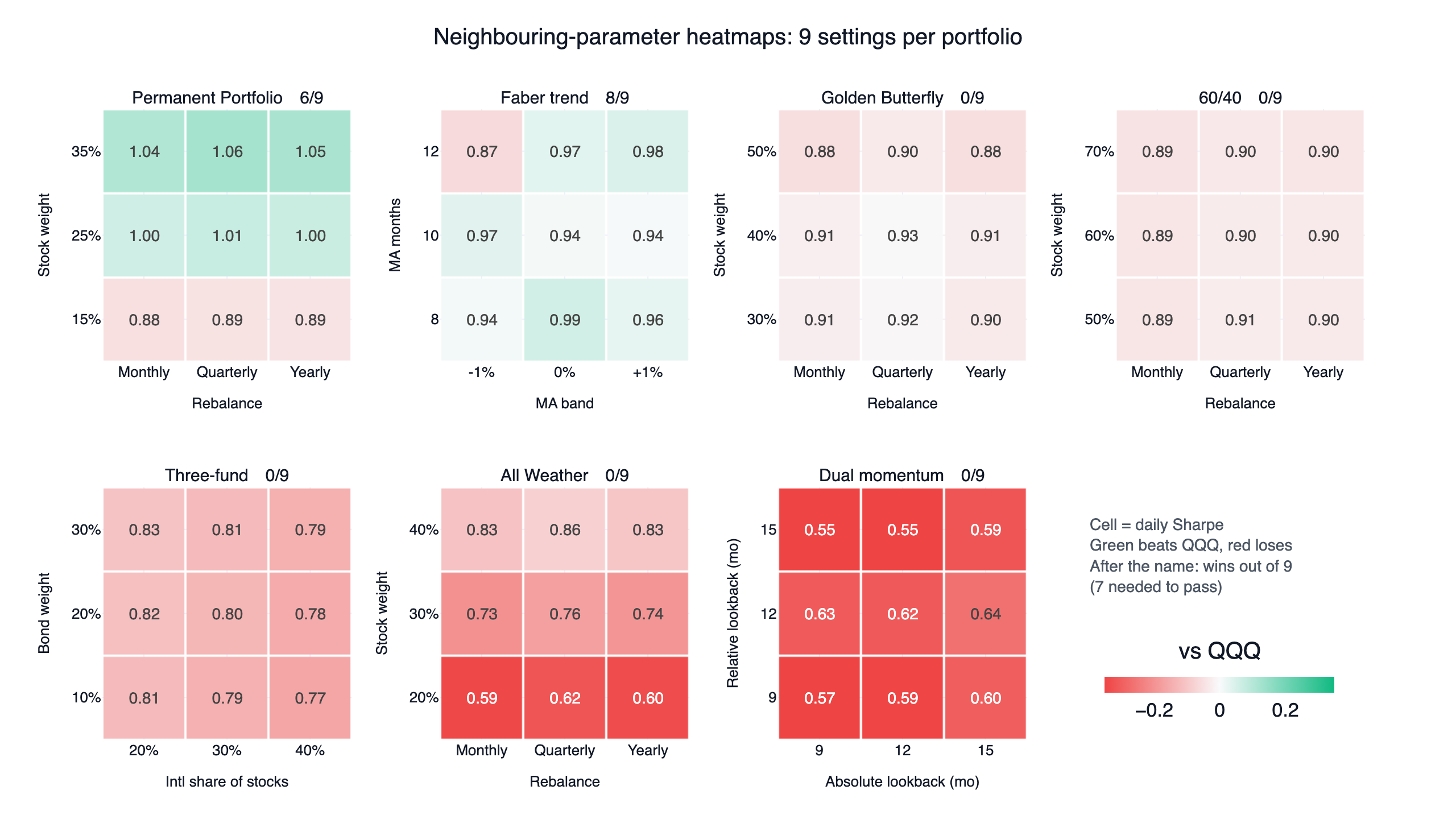
Each block is one portfolio's 3×3 grid; the number in each cell is its daily Sharpe, green beats QQQ and red loses. Fourteen of the 63 cells win, and all fourteen belong to two portfolios.
The Permanent Portfolio grid splits horizontally. All six settings with 25% or 35% in stocks win (1.00 to 1.06); all three with 15% lose (0.88 to 0.89). Rebalancing frequency barely matters: the three cells in a row differ by less than 0.02. So the edge has little to do with the four-way equal split. It comes from stocks and gold both doing well in this window (VTI 14.5% a year, GLD 12.8%) while long Treasuries lost money (TLT -1.0% a year) and T-bills earned 2.4%; the less stock you hold, the more that hurts.
Faber's trend model is the only portfolio to pass this check, with eight of nine settings ahead and a range of 0.87 to 0.99. The one loser is the 12-month average held as long as price stays above 99% of it, the slowest exit in the grid. The averages for the three lengths differ by less than 0.03, so the grid shows no clear preference for a faster or slower filter.
The other five portfolios win zero cells. The nine 60/40 settings sit between 0.89 and 0.91 and barely respond to the parameters. All Weather climbs from 0.59 to 0.86 as its stock weight rises. The three-fund portfolio loses Sharpe as the international share grows (VXUS returned 9.0% a year against 14.5% for VTI). Dual momentum stays between 0.55 and 0.64 whatever the lookbacks.
Result 2: the two halves tell different stories
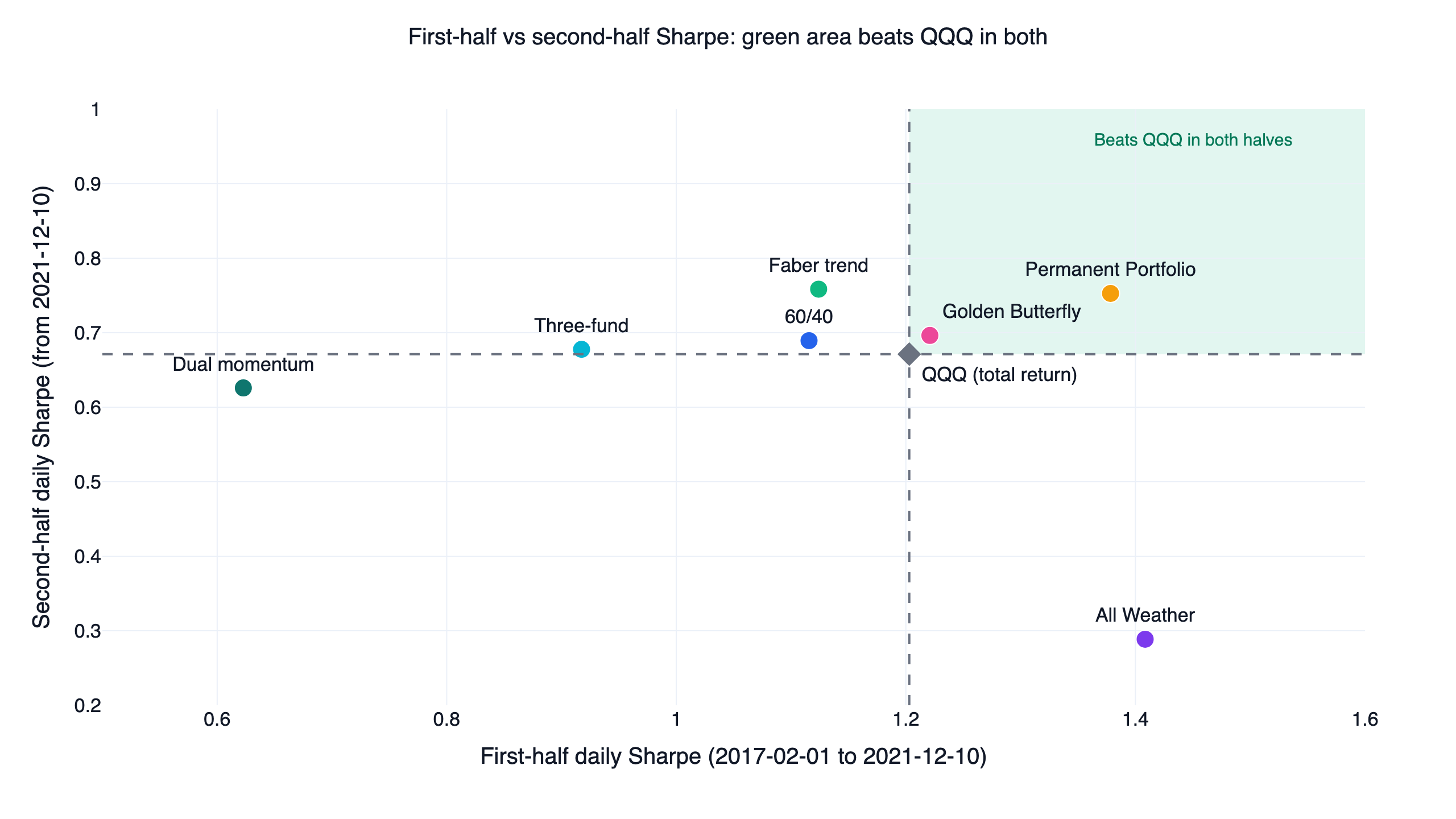
QQQ's daily Sharpe was 1.20 in the first half (2017-02-01 to 2021-12-10) and 0.67 in the second (2021-12-10 to 2026-10-27). A portfolio has to land in the green area to pass.
- All Weather was the strongest portfolio in the first half (1.41) and the weakest in the second (0.29). It holds 55% in intermediate and long Treasuries. In the first half rates rose in 2017 and 2018, then fell sharply in 2019 and 2020, ending lower overall; and TLT returned 6.9% a year while hedging stocks; in the second half rates jumped, TLT returned -8.3% a year (-31.2% in 2022 alone), and All Weather lost 19.7% in 2022.
- The Permanent Portfolio and the Golden Butterfly are the only two that won both halves, helped by gold returning 17.9% a year in the second half (7.9% in the first). The Golden Butterfly still lost the full period (0.930 against 0.934) and all nine settings, so this is the only check it passed.
- Faber, 60/40 and three-fund all fell short of QQQ's 1.20 in the first half, when QQQ compounded at 27.8% a year and every dollar held outside large US growth stocks fell behind. In the second half QQQ slowed to 13.6% a year and all three beat it (0.76, 0.69 and 0.68 against 0.67).
- Dual momentum lost both halves (0.62 and 0.63).
Result 3: far smaller drawdowns, far lower returns
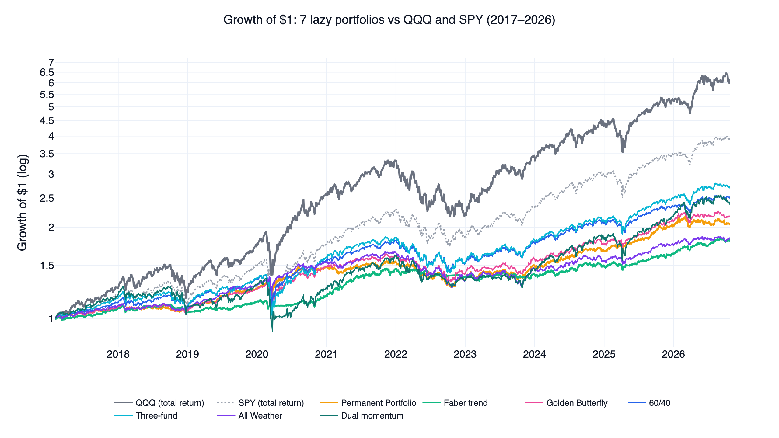
One dollar in QQQ became 3.94. The seven portfolios ended between 2.73: three-fund 2.53, dual momentum 2.18, Permanent 1.85 and Faber $1.81. Even the highest CAGR, the three-fund portfolio's 10.9%, is little more than half of QQQ's 20.5%.
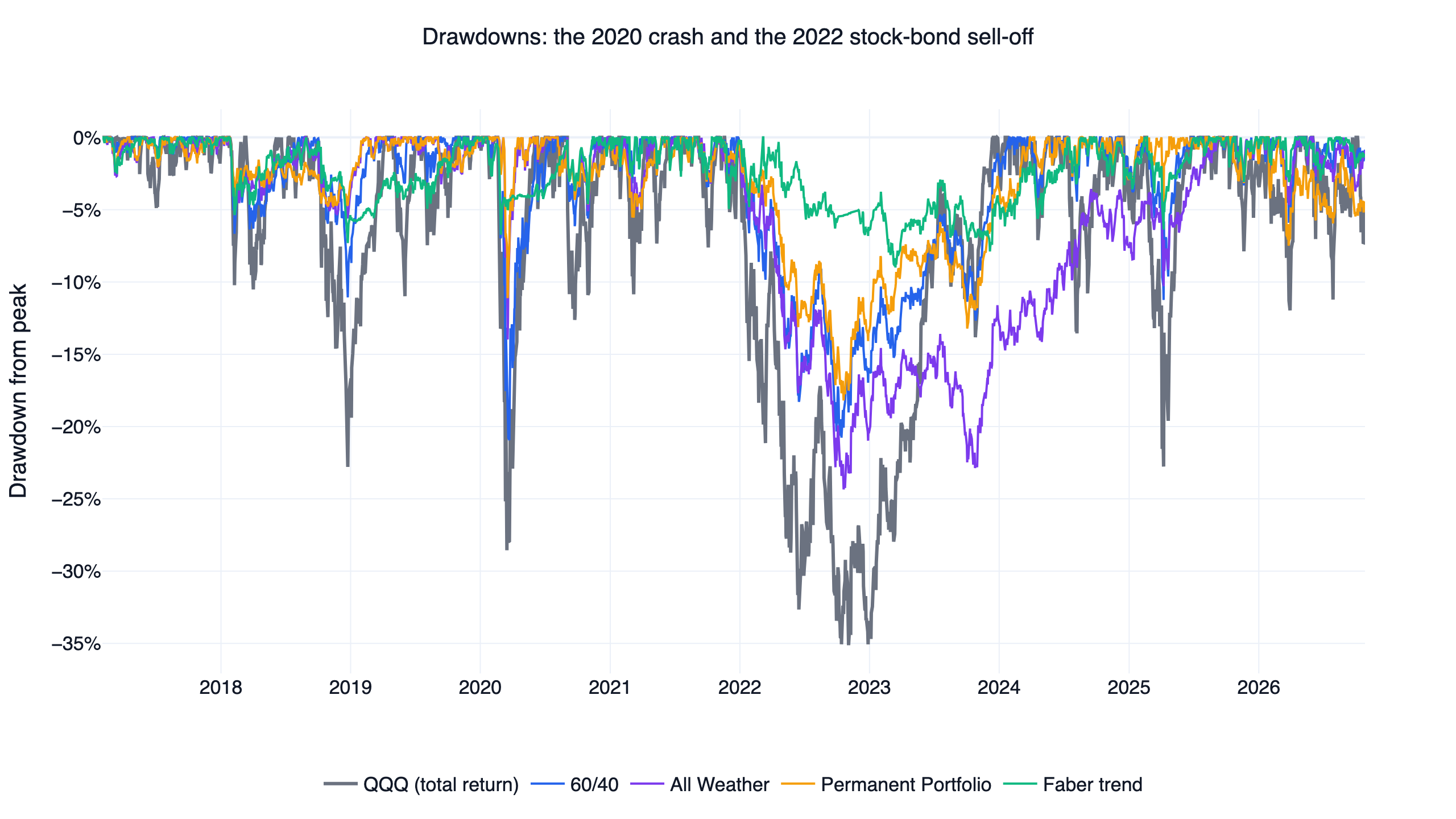
What the lower returns bought was shallower drawdowns. QQQ's -35.1% maximum drawdown came in 2022. That year 60/40 lost 15.9%, the Permanent Portfolio 13.1%, and Faber only 5.7%. Faber's worst drawdown over the whole window was -9.0%. Faber paid for that protection. At the end of February 2020, US stocks, foreign stocks and REITs fell below their averages; commodities had already been out since January, so 80% of the portfolio sat in T-bills. US stocks only climbed back above their average at the end of May, and the model began re-entering in early June, missing most of the rebound: it made 5.0% in 2020 while QQQ made 48.6%. In 2023, when QQQ rose 54.9%, Faber rose 2.1%. Dual momentum shows the opposite failure. It still held SPY through the whole March 2020 crash, switched to bonds at the end of that month and then missed April's rebound, so its maximum drawdown of -33.7% matched SPY's. At the end of May 2022 it rotated from stocks into bonds just as bonds kept falling, and it lost 17.2% that year.
Why they lose: after late 2021, bonds stopped hedging stocks
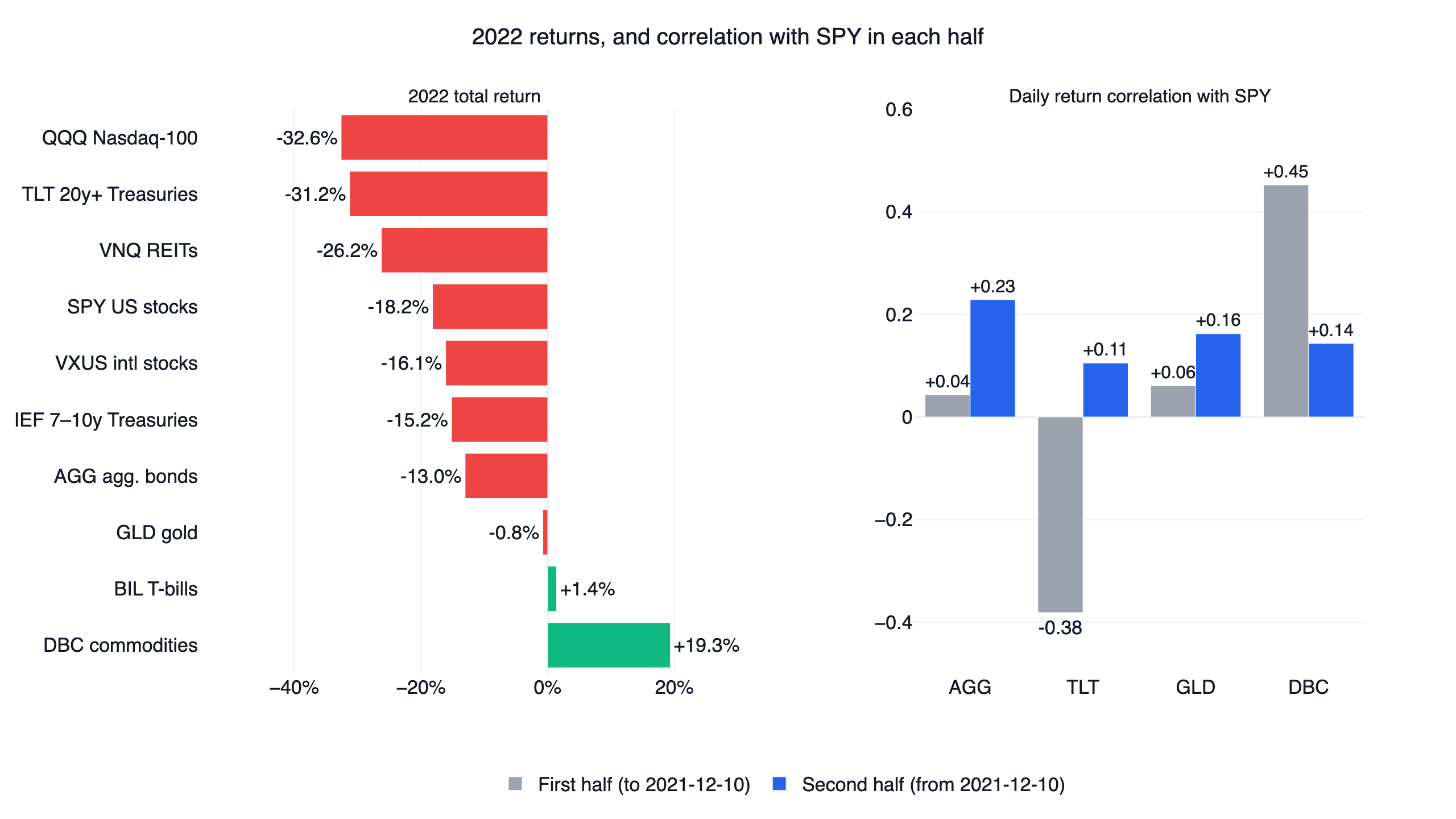
Two things explain most of the gap.
The negative stock-bond correlation disappeared in the second half. Every one of these designs assumes bonds rise when stocks fall. In the first half, TLT's daily correlation with SPY was -0.38, a real hedge; after 2021-12-10 it was +0.11, AGG's rose from +0.04 to +0.23 and gold's from +0.06 to +0.16, while commodities (DBC) fell from +0.45 to +0.14. In 2022 SPY lost 18.2% and QQQ 32.6%, and bonds did not catch the fall: AGG lost 13.0%, IEF 15.2% and TLT 31.2%. VNQ, one of Faber's five asset classes, lost 26.2% (the trend rule kept Faber out of it for most of the year), and the three-fund portfolio's international sleeve (VXUS) lost 16.1%. The only offsets left were commodities (DBC +19.3%), T-bills (BIL +1.4%) and roughly flat gold (-0.8%). Campbell, Sunderam & Viceira (2009) explain the mechanism: the sign of the stock-bond correlation depends on the role of inflation, and when inflation is the main risk, rising rates push stocks and bonds down together. Their data show the covariance between Treasuries and stocks was clearly positive in the early 1980s and turned negative only in the 2000s.
This was the Nasdaq-100's decade. QQQ compounded at 20.5% a year, total-market VTI at 14.5%, international VXUS at 9.0%, and US aggregate bonds (AGG) at 1.7%. Any allocation that moves money out of large US growth stocks starts behind. Gold (12.8%) was the only diversifier that closed some of the distance. Daily Sharpe credits them for lower volatility, but in most cases that did not make up for the lower return.
One more caveat: our Sharpe convention actually flatters these portfolios. The daily Sharpe here deducts no risk-free rate. Deduct the T-bill return (BIL) and QQQ's daily Sharpe becomes 0.83, while the Permanent Portfolio drops to 0.70, 60/40 to 0.69 and Faber to 0.59: all seven lose to QQQ. A large share of a low-volatility portfolio's return is T-bill interest, and removing it widens the gap.
The code
The snippet below builds 60/40 and Faber's model, then compares each with QQQ over the same trading days. The full strategy.py runs all seven portfolios, the 63 neighbouring settings, both halves and the cost stress test, and writes every number in this article.
Show Code
import pandas as pd
from finlab import data
from finlab.backtest import sim

data.set_market("us_fund")
close = pd.DataFrame(data.get("us_fund_price:adj_close"))
close = close[close["SPY"].notna()]  # keep US trading days only

# 1. Fixed weights: 60/40, rebalanced every quarter
weights = pd.DataFrame({"SPY": 0.6, "AGG": 0.4}, index=close.index)
sixty_forty = sim(weights.loc["2016-12-30":], resample="Q", trade_at_price="close", upload=False)

# 2. Faber trend: five assets at 20% each; below the 10-month average -> T-bills
assets = ["SPY", "EFA", "IEF", "VNQ", "DBC"]
month_ends = close.index.to_series().groupby(close.index.to_period("M")).max()
monthly = close.loc[month_ends.values, assets]
in_trend = monthly > monthly.rolling(10).mean()
position = in_trend.astype(float) * 0.2
position["BIL"] = 1 - position.sum(axis=1)
faber = sim(position.loc["2016-12-30":], resample="M", trade_at_price="close", upload=False)

# 3. Daily Sharpe versus QQQ (total return) over the same days
def daily_sharpe(curve):
    returns = curve.pct_change().dropna()
    return returns.mean() / returns.std() * 252 ** 0.5

days = close.loc["2017-02-01":].index
qqq = round(daily_sharpe(close["QQQ"].loc[days]), 2)
for name, report in [("60/40", sixty_forty), ("Faber", faber)]:
    curve = report.creturn.reindex(days)
    print(name, round(daily_sharpe(curve), 2), "QQQ", qqq)
In our environment this prints 0.90 for 60/40, 0.94 for Faber and 0.93 for QQQ, matching the full script. Run finlab.login() first; the package walks you through signing in.
Run it with your AI agent
The fastest way to test your own mix is to let an AI coding agent edit and rerun the script. Install the FinLab skill with npx skills add https://github.com/koreal6803/finlab-ai --skill finlab; it works with Claude Code, Codex and Gemini CLI, and the agent setup page covers each one. Then ask for one change at a time, for example "move the Permanent Portfolio's cash into SHY" or "add a 10-month trend filter to 60/40", and have it rerun all three checks before you trust the new curve. If you prefer not to install anything, the same research runs in FinLab Studio at studio.finlab.finance through the AI-assisted setup.
Backtest method and limits
| Item | How this study handles it |
|---|---|
| Window | 2017-02-01 to 2026-10-27. ETF prices start in January 2016; dual momentum's first 12-month signal is available at the end of January 2017, so the comparison starts on February 1. Fixed-weight portfolios and Faber's model take positions at the end of December 2016, and only returns from February 1 on are compared. The five dual momentum grid settings with a 15-month lookback start on 2017-05-01 and are compared with QQQ over those days (daily Sharpe 0.90) |
| Data | finlab us_fund_price:adj_close, closes adjusted for reinvested distributions. The table contains a few dozen empty rows on US market holidays; we drop them first, otherwise a holiday that falls on a month end (such as May 31, 2021) breaks the moving average. Run with finlab 2.2.21; earlier versions could trade on those holiday rows and give slightly different numbers |
| Execution | Signals and rebalances use the month-end (or quarter-end, year-end) close and trade at the next day's close; no data from after the signal is used (look-ahead bias) |
| Costs | finlab's US default: no commission, no tax, no bid-ask spread. Under the 0.1%-per-side stress test the fixed-weight portfolios lose 0.01 to 0.02 percentage points of CAGR, Faber falls from 6.3% to 5.9%, and dual momentum from 9.5% to 9.0% |
| Turnover | Backing out turnover from the 0.1%-per-side cost drag, the fixed-weight portfolios trade roughly 6% to 10% of the portfolio (one way) a year, Faber about 200% and dual momentum about 210%. Faber changed its target weights at 66 of 117 month ends; dual momentum switched holdings 19 times in 117 months |
| ETF choice | The most liquid common ETF for each asset class. The original papers use indices (Faber uses the GSCI commodity index; we use DBC). ETF fees are already in the adjusted prices |
| Dividend withholding | Adjusted prices assume every distribution is reinvested in full; no tax is deducted. For non-US investors, stock and REIT ETF distributions are withheld at 30% (or a treaty rate); interest-related dividends from US bond ETFs are usually exempt, depending on the broker. REIT-heavy portfolios are affected most |
| Benchmark | QQQ buy-and-hold with dividends reinvested, no costs; SPY as a reference |
| Sample | Every result is in-sample; the halves are a stability check, not out-of-sample validation. Nine years and nine months cover only one shift from falling to rising rates |
What this result does and does not say
Under this setup, from 2017 to 2026, none of seven classic asset allocation portfolios reliably beat simply holding QQQ on risk-adjusted terms. That does not make them useless. Their stated goal is to shrink drawdowns so an investor can stay invested through a bear market, and all seven did have shallower drawdowns than QQQ: Faber's was about a quarter of QQQ's, the Permanent Portfolio's and the Golden Butterfly's about half. Someone who would sell everything at -35% might well earn more holding a portfolio that only falls 18%, and no backtest can measure that.
Nor does it say the next decade will repeat. This window contains an unusually long run for large US growth stocks and the fastest rate-hiking cycle in four decades; Faber's 2013 update of his paper and Antonacci's book both use data from the 1970s on, covering that decade's inflation plus the 2000 and 2008 bear markets. None of the seven uses optimization, and that is part of their appeal: DeMiguel, Garlappi & Uppal (2009) found that none of 14 optimized models consistently beat naive 1/N diversification out of sample, because estimation error wipes out the gains from optimizing.
Who this is useful for: investors who want a passive ETF allocation, care more about drawdowns than about maximum return, and can accept trailing a stock index. Who it is not for: anyone whose goal is to beat the Nasdaq-100, or who cannot sit through years of lagging the market. For the opposite approach, a QQQ risk-on/risk-off signal applied to leveraged index ETFs, see the ETF rotation strategy backtest and the US quant trading strategies overview; the low-volatility strategy takes a defensive route inside equities instead.
FAQ
Does the All Weather portfolio still work? In the simplified retail version (30% stocks, 55% Treasuries, 7.5% each in gold and commodities), it had a 0.76 daily Sharpe from 2017 to 2026, second-lowest of the seven. It did very well before 2022 (1.41 in the first half) and only 0.29 in the second half after long Treasuries collapsed. Levered institutional risk parity would behave differently; we did not test it.
How did the Permanent Portfolio backtest? It had the highest full-period daily Sharpe of the seven, 1.01 against QQQ's 0.93, with a 7.7% CAGR and a -18.2% maximum drawdown, and it beat QQQ in both halves. It failed the parameter check: all three settings with 15% in stocks lost, so the result depends on how strong stocks and gold were in this window.
Is the 60/40 portfolio dead? Over this window 60/40 compounded at 10.0% with a 0.90 daily Sharpe, and all nine settings (50% to 70% stocks, monthly to yearly rebalancing) landed between 0.89 and 0.91: very stable, and consistently just behind QQQ. In 2022 it fell 15.9% as stocks and bonds dropped together, a scenario its design did not anticipate.
What is the difference between the Golden Butterfly and the Permanent Portfolio? The Golden Butterfly replaces all cash with short-term Treasuries (SHY), raises stocks from 25% to 40% (half of it small-cap value, VBR), and cuts long Treasuries and gold to 20% each. With more in stocks it compounded faster (8.4% against 7.7%), but small-cap value lagged the total market (9.5% against 14.5% a year) and added volatility, so its daily Sharpe was lower (0.930 against 1.01).
How much international stock should a three-fund portfolio hold? In our nine settings, a higher international share always meant a lower daily Sharpe: with 20% bonds, an international share of 20%, 30% and 40% gave 0.82, 0.80 and 0.78. That reflects US stocks' large lead from 2017 to 2026, not a forecast.
Why compare against QQQ rather than 60/40 or SPY? QQQ with dividends reinvested is the benchmark FinLab uses for all US research, so results stay comparable across articles. Against SPY, the Permanent Portfolio (1.01), Faber (0.94), the Golden Butterfly (0.93) and 60/40 (0.90) all have higher daily Sharpe than SPY's 0.87, but that is not the test used here. The first chart shows both benchmarks.
How often should an asset allocation be rebalanced? Across the four portfolios where we varied it (60/40, All Weather, Permanent, Golden Butterfly), monthly, quarterly and yearly rebalancing changed daily Sharpe by less than 0.03, far less than the choice of stock weight.
Reproduce it yourself
- strategy.py: the full test, seven portfolios, 63 neighbouring settings, both halves and the cost stress test. Edit the weights in
FIXEDto test your own mix. - data.csv: daily equity curves of the seven portfolios, QQQ and SPY from 2017-02-01.
- metrics.json: every statistic quoted in this article, including all 63 settings, calendar-year returns and correlations.
More US research is on the FinLab blog, including the same three checks applied to ten academic stock factors and an introduction to factor investing. The team behind it is on the about page, and examples of what users build are on use cases.
Last updated: 2026-10 | Backtest window: 2017-02 to 2026-10 | Benchmark: QQQ total return | Author: FinLab Quant Research (reviewed by a quantitative researcher)
Past performance is not indicative of future results, and every result here is an in-sample backtest. This content is for education only and does not constitute investment advice.
FinLab AI
Want to build your own strategy?
Describe your stock-picking ideas in natural language. AI automatically validates, backtests, and gives you answers
Start Free