Run this strategy
Copy the prompt to reproduce the evidence above with the article’s data, assumptions, and risk checks.
Tell your AI:
Set up FinLab and rerun the ten US factor portfolios against QQQ. Please read: https://finlab.finance/en/setup?relatedUrl=/en/blog/us-academic-factors-backtest
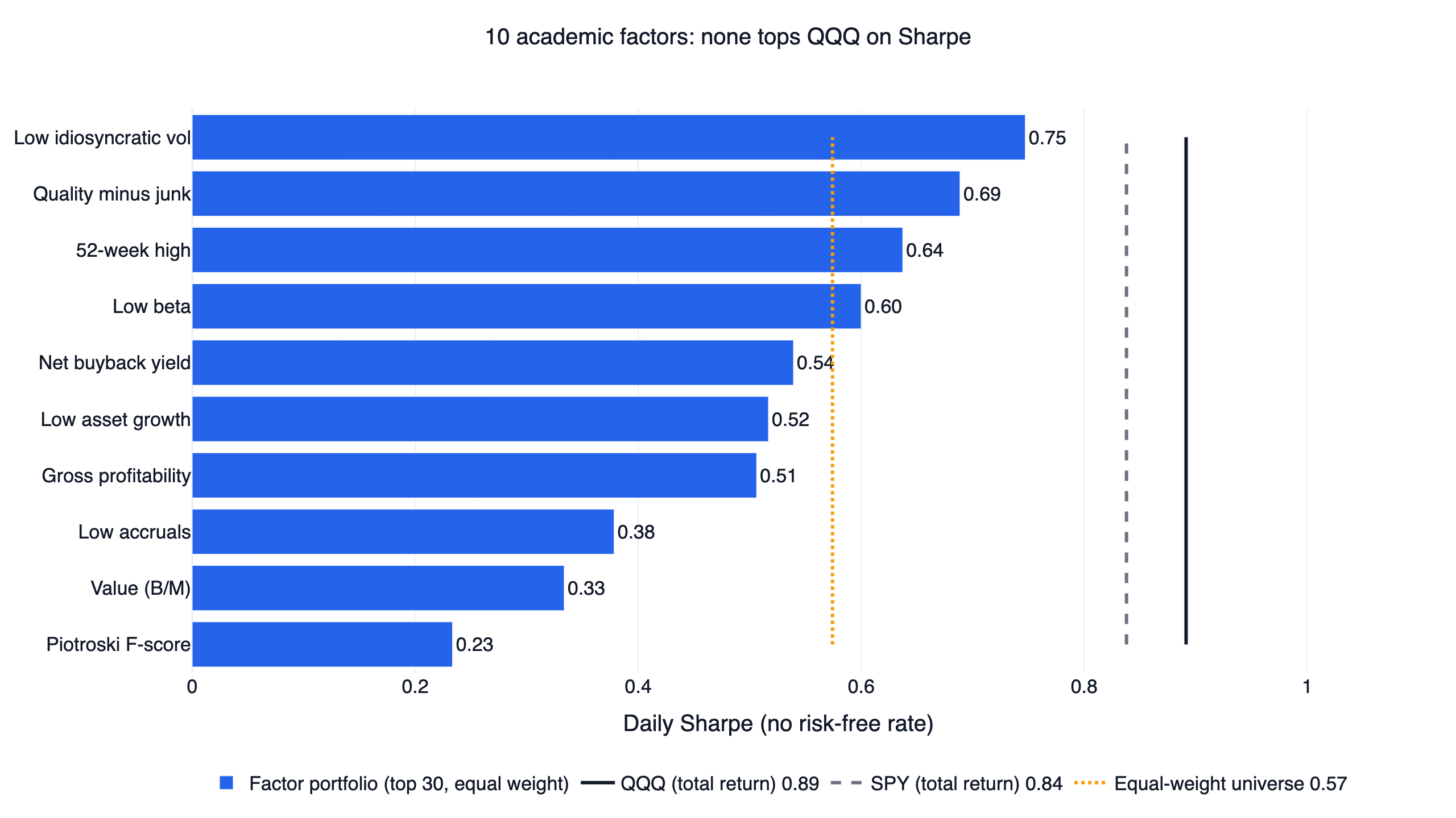
We rebuilt ten published stock factors on US equities and held each as a long-only, 30-stock portfolio from August 2017 to October 2026. None matched QQQ on risk-adjusted return: the best base setting reached a daily Sharpe of 0.75 (low idiosyncratic volatility) against 0.89 for QQQ with dividends reinvested, and the best of all 90 neighbouring parameter settings reached 0.83. The factors come from the papers most cited in asset pricing: value, gross profitability, asset growth, accruals, share buybacks, the 52-week high, low beta, low idiosyncratic volatility, the Piotroski F-score, and quality minus junk. Each one had to clear three checks to count as working. None cleared even the first. That makes this a test of a specific question, "would a stock-picking factor have beaten simply owning QQQ over the last nine years?", and the answer for all ten is no.
The ten factors at a glance
| Factor (paper) | Daily Sharpe | CAGR | Max drawdown | Settings beating QQQ | First / second half Sharpe |
|---|---|---|---|---|---|
| Value, book-to-market (Fama & French 1992) | 0.33 | 5.7% | -70.9% | 0 / 9 | 0.24 / 0.47 |
| Gross profitability (Novy-Marx 2013) | 0.51 | 9.9% | -45.0% | 0 / 9 | 0.48 / 0.54 |
| Low asset growth (Cooper, Gulen & Schill 2008) | 0.52 | 10.9% | -49.2% | 0 / 9 | 0.44 / 0.60 |
| Low accruals (Sloan 1996) | 0.38 | 7.4% | -61.1% | 0 / 9 | 0.46 / 0.30 |
| Net buyback yield (Pontiff & Woodgate 2008) | 0.54 | 11.6% | -51.4% | 0 / 9 | 0.48 / 0.61 |
| 52-week high (George & Hwang 2004) | 0.64 | 10.8% | -27.8% | 0 / 9 | 0.75 / 0.51 |
| Low beta (Frazzini & Pedersen 2014) | 0.60 | 9.3% | -31.9% | 0 / 9 | 0.71 / 0.46 |
| Low idiosyncratic volatility (Ang et al. 2006) | 0.75 | 10.7% | -35.8% | 0 / 9 | 0.70 / 0.90 |
| Piotroski F-score (Piotroski 2000) | 0.23 | 2.7% | -68.6% | 0 / 9 | -0.12 / 0.75 |
| Quality minus junk (Asness, Frazzini & Pedersen 2019) | 0.69 | 12.3% | -35.9% | 0 / 9 | 0.59 / 0.79 |
| QQQ, total return | 0.89 | 19.7% | -35.1% | benchmark | 0.90 / 0.88 |
| SPY, total return | 0.84 | 14.8% | -33.7% | reference | not split |
| Equal-weight liquid universe | 0.57 | 10.5% | -41.4% | reference | 0.57 / 0.59 |
All portfolios start on 2017-08-01 and end on 2026-10-26; QQQ and SPY are buy-and-hold with dividends reinvested over the same days. The half-window QQQ Sharpe is 0.90 for the first half and 0.88 for the second.
How a factor had to pass
"Beat" has one meaning in this study: a higher daily Sharpe ratio than QQQ total return over exactly the same trading days. Sharpe is mean daily return over its standard deviation, annualised with √252, without subtracting a risk-free rate. (The US strategy comparison reports monthly Sharpe, on which QQQ scores 1.09, so its figures are not directly comparable with these.) A factor counted as working only if it passed all three checks:
- A plateau, not a peak. Each factor's two main parameters were set to a base value and one neighbour on each side, giving nine settings. At least seven of the nine (70%) had to beat QQQ. For the five pure accounting ratios and quality minus junk the two parameters are universe size (500, 1,000, 1,500 most liquid stocks) and holdings (20, 30, 50). For the three price factors they are the lookback window and holdings: 189, 252 and 315 days for the 52-week high, 126, 252 and 378 for low beta, and 10, 21 and 42 for low idiosyncratic volatility, whose base is the paper's one-month window. For the F-score they are the cheap-stock share (top 20%, 30%, 40% by book-to-market) and the minimum score (7, 8, 9).
- Both halves. The window was cut at its midpoint, 2022-03-15. The base setting had to beat QQQ in each half separately, so a factor cannot pass on one lucky stretch.
- Costs included. Every run uses finlab
sim()with its default US cost model (USMarket: zero commission, no transfer tax), the norm at commission-free US brokers. No cost was switched off to help a result.
The first check is where all ten failed: across the 90 settings, the number that beat QQQ was zero.
The ten factors and how each was built
Every factor below is computed from FinLab's US tables. Fundamentals come from us_income_statement, us_balance_sheet, and us_cash_flow, which FinLab dates by the SEC filing date, so a number only enters the score after the 10-Q or 10-K is public. Each month the portfolio buys the 30 highest-scoring stocks in the liquid universe at the next day's close.
- Value, book-to-market. Fama & French (1992) found that stocks with high book equity relative to market value earned higher average returns. Score: latest stockholders' equity divided by daily market cap; negative book value is excluded.
- Gross profitability. Novy-Marx (2013) showed that gross profit scaled by total assets predicts returns about as well as book-to-market, and works as a hedge for value. Score: trailing-four-quarter gross profit divided by total assets.
- Low asset growth. Cooper, Gulen & Schill (2008) documented that firms growing their balance sheet fastest went on to underperform. Score: the negative of year-over-year total asset growth.
- Low accruals. Sloan (1996) found that earnings backed by cash persist while earnings made of accruals reverse. We use the cash-flow definition recommended by Hribar & Collins (2002): trailing net income minus operating cash flow, divided by average total assets; low is good.
- Net buyback yield. Pontiff & Woodgate (2008) linked share issuance to lower future returns, and Ikenberry, Lakonishok & Vermaelen (1995) found positive drift after buyback announcements. Score: the negative of trailing net common stock issuance, divided by market cap, so net repurchasers rank highest.
- 52-week high. George & Hwang (2004) showed that stocks trading close to their 52-week high keep outperforming. Score: adjusted close divided by the highest adjusted close of the last 252 trading days.
- Low beta. Frazzini & Pedersen (2014) built "betting against beta" from leveraged low-beta stocks and shorted high-beta stocks. A long-only investor can only hold the low-beta leg, so that is what we test: 252-day beta of daily returns against SPY, lowest first.
- Low idiosyncratic volatility. Ang, Hodrick, Xing & Zhang (2006) found that stocks with high residual volatility earn strikingly low returns. Score: the standard deviation of 21-day residuals from a one-factor regression on SPY (the paper uses the three Fama-French factors); lowest first.
- Piotroski F-score. Piotroski (2000) scored cheap stocks on nine accounting signals and bought the ones scoring 8 or 9 within the highest book-to-market fifth. Our base setting widens the cheap pool to the top 30% (the 20% version is in the parameter grid) and holds every stock with an F-score of at least 8, equal weight, so the number of holdings floats with the count.
- Quality minus junk. Asness, Frazzini & Pedersen (2019) define quality as profitability, growth, safety, and payout. We average ranks of six profitability measures, their one-year changes (the paper uses five-year changes, which our 2016 start cannot support), three safety measures (low beta, low leverage, low earnings volatility), and net buyback yield.
Result 1: the base settings trail QQQ by a wide margin
The chart at the top ranks the ten base portfolios by Sharpe. Low idiosyncratic volatility (0.75), quality minus junk (0.69) and the 52-week high (0.64) come closest, but all three sit well below QQQ's 0.89. Value is near the bottom at 0.33 with a -70.9% maximum drawdown, and the Piotroski F-score portfolio, which concentrates in the cheapest stocks, finished last at 0.23.
The useful reference line is the orange one: an equal-weight portfolio of the entire liquid universe, rebalanced monthly, scored 0.57. Four of the ten factors beat that line (the 52-week high, low beta, low idiosyncratic volatility, and quality minus junk), so the strongest factors did improve on the average stock. The problem is the distance between the average US stock and QQQ, which is larger than anything a factor tilt added.
Result 2: no plateau anywhere in 90 settings
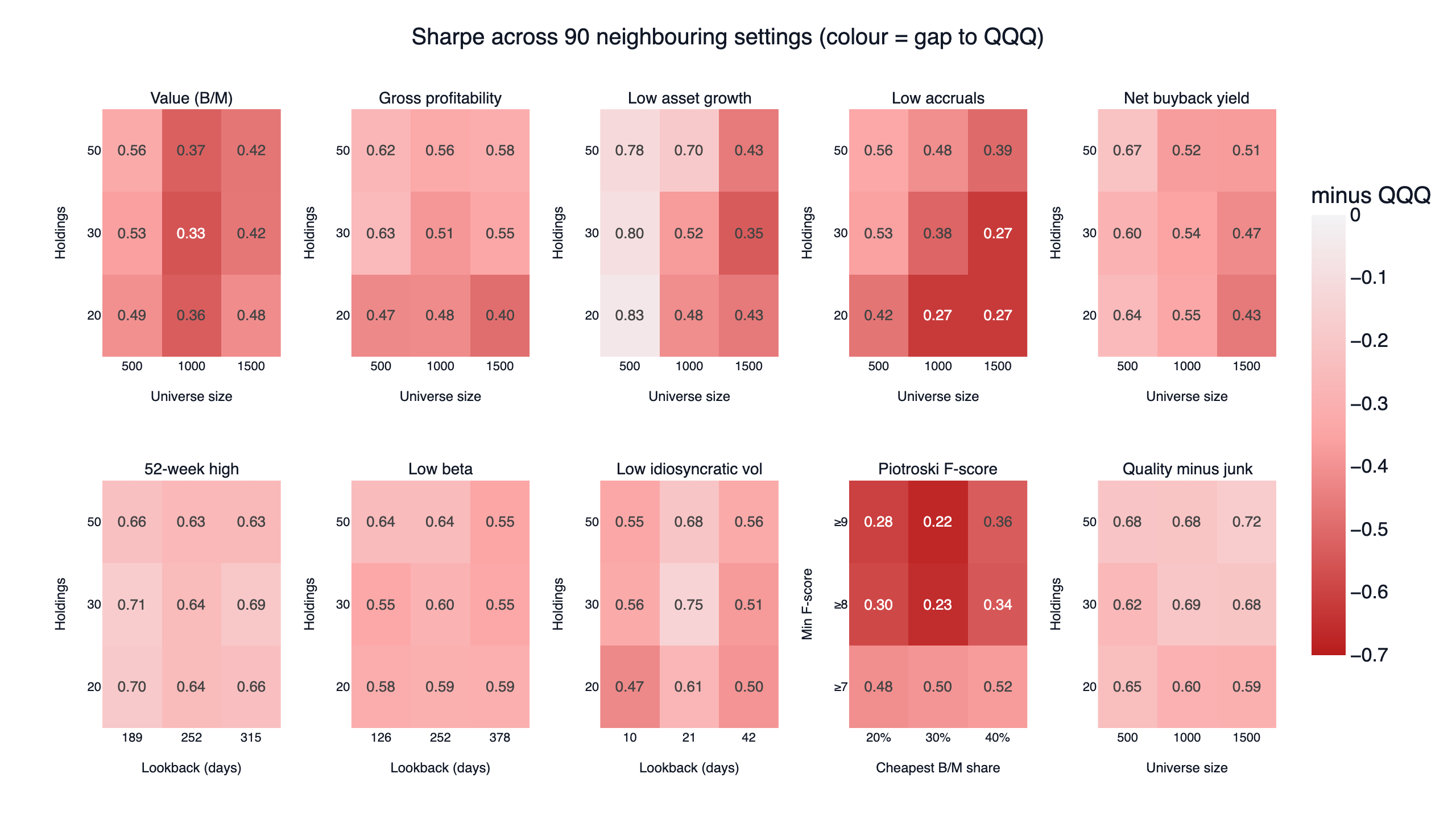
Each small grid is one factor; the number in each cell is that setting's Sharpe and the colour is the gap to QQQ. Every one of the 90 cells is below QQQ. The closest any single setting came was low asset growth in the 500-stock universe with 20 holdings, at 0.83, and that factor's whole 500-stock column sits between 0.78 and 0.83. It looks like a plateau until you read across: with 1,000 or 1,500 stocks the same factor drops to 0.35-0.70, so the near-miss depends on restricting the test to the largest companies, the part of the market QQQ already owns. All five accounting ratios had their best setting in the 500-stock universe. The 52-week high (0.63-0.71) and low beta (0.55-0.64) were the most stable, followed by quality minus junk (0.59-0.72); low idiosyncratic volatility ranged from 0.47 to 0.75 depending on the lookback. All of them were stable well below the bar.
Result 3: the halves tell the same story
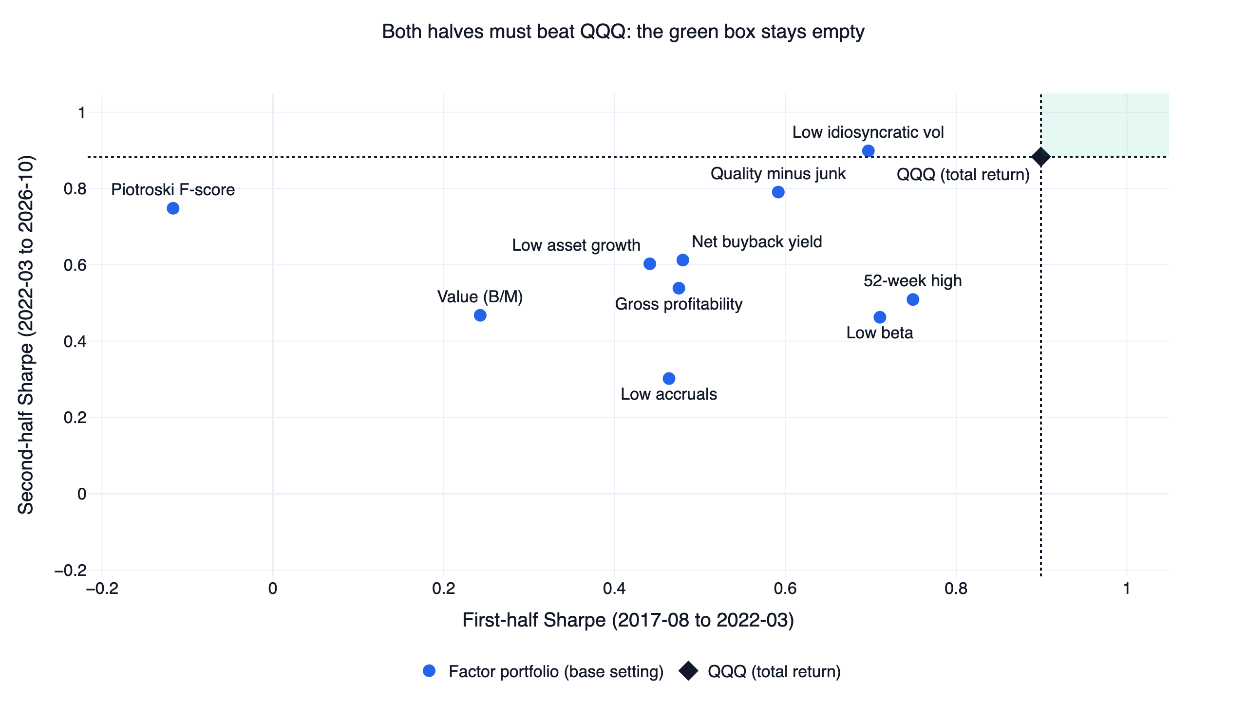
To pass, a factor had to land in the green box: above QQQ's first-half Sharpe (0.90) and above its second-half Sharpe (0.88). The box is empty. The 52-week high and low beta were the strongest first-half portfolios (0.75 and 0.71) and weakened after March 2022. Low idiosyncratic volatility did the reverse: 0.70 in the first half and 0.90 in the second, the only base portfolio that beat QQQ (0.88) in either half. The Piotroski F-score had a negative first-half Sharpe (-0.12) and 0.75 in the second half, the value factor's own path through the 2020 crash and the 2022 rotation, amplified.
Why they lose: the benchmark is the hard part
Three things explain most of the shortfall.
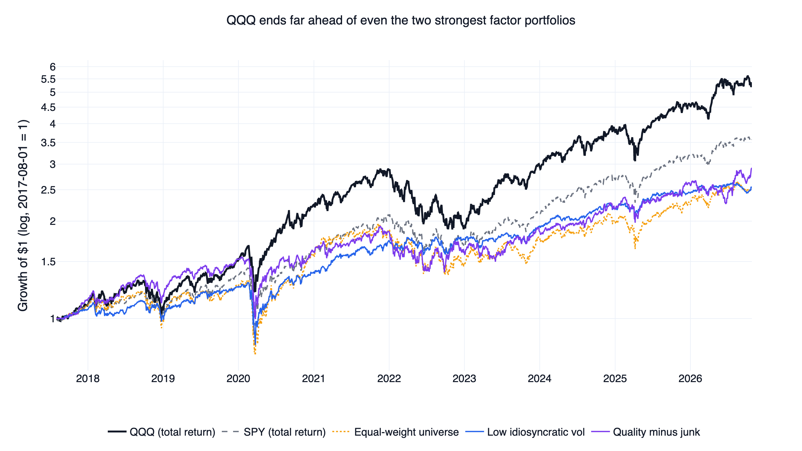
The decade belonged to the largest companies. QQQ compounded at 19.7% a year, SPY at 14.8%, and the equal-weight liquid universe at 10.5%. A long-only factor portfolio of 30 equal-weighted stocks starts from the equal-weight universe, not from QQQ. The two strongest portfolios show what that means: quality minus junk compounded 1.8 points a year faster than the equal-weight universe (12.3% against 10.5%), and low idiosyncratic volatility matched the universe's return with far less volatility (15.2% a year against 21.4%). One dollar still grew to about 2.6 respectively, against $5.3 in QQQ.
The factor premiums themselves were small. Inside the same universe we sorted stocks into deciles every month and measured the return gap between the best and worst decile. Six of the ten factors had a positive top-minus-bottom spread, led by gross profitability (+6.5% a year) and low accruals (+6.0%), but none had a t-statistic above 1.4. Value's spread was essentially zero (-0.2%), and low beta's was -7.1%: the highest-beta decile out-earned the lowest. The full decile analysis is in the factor investing overview. This matches the replication literature: McLean & Pontiff (2016) found anomaly returns are 58% lower after publication, about 32 points of which they attribute to investors trading on the published result, and Hou, Xue & Zhang (2020) found that most anomalies lose significance once micro-caps no longer dominate the averages. Our universe of the 1,000 most liquid names, each trading over $5M a day, keeps micro-caps out in a similar way.
Low risk was the wrong side of a bull market. Low beta and low idiosyncratic volatility were the two least volatile portfolios of the ten (17.3% and 15.2% a year, against 23.3% for QQQ), but in a market that rewarded high-beta growth they gave up too much return. Much of the return in Frazzini & Pedersen (2014) comes from shorting high-beta stocks, and in this window the highest-beta decile earned the most (a -7.1% decile spread), so the long-only low-beta leg lost even on a risk-adjusted basis.
The code
The core of the test fits in a few steps. This excerpt builds the universe, scores one factor (gross profitability), holds the top 30, and compares the result with QQQ; the full strategy.py runs all ten factors, the 90-setting grid, and the decile test.
Show Code
from finlab import data
from finlab.backtest import sim

data.set_market("us")

# 1. Liquid universe: top 1,000 by 60-day dollar volume, price > $5.
#    (strategy.py also keeps only common stocks, drops ADRs and financials,
#    and skips stocks for a year after a +/-50% day.)
close = data.get("us_price:close")
volume = data.get("us_price:volume")
dollar_volume = (close * volume).rolling(60, min_periods=20).mean()
universe = dollar_volume.is_largest(1000) & (dollar_volume > 5e6) & (close > 5)

# 2. Gross profitability (Novy-Marx 2013): trailing gross profit / total assets.
#    Statement items are dated by SEC filing date, so no extra shift is needed.
gross_profit = data.get("us_income_statement:gross_profit").rolling(4).sum()
total_assets = data.get("us_balance_sheet:total_assets")
score = gross_profit / total_assets

# 3. Hold the 30 best-scoring stocks, equal weight, rebalanced monthly.
position = score[universe].is_largest(30)
report = sim(position.loc["2017-08-01":], resample="M", upload=False)

# 4. Compare with QQQ (total return) over the same days.
qqq = data.get("us_fund_price:adj_close")["QQQ"].reindex(report.creturn.index).ffill()
for name, curve in [("strategy", report.creturn), ("QQQ", qqq / qqq.iloc[0])]:
    daily = curve.pct_change().dropna()
    print(name, round(daily.mean() / daily.std() * 252 ** 0.5, 2))
Hand the script to an AI agent with the FinLab skill installed and ask it to change one thing at a time, such as a different holding count or a sector-neutral version, then rerun the three checks before trusting any single curve.
Backtest method and limits
| Item | How it was handled |
|---|---|
| Window | 2017-08-01 to 2026-10-26. Prices start in 2016 and statements in 2016, so August 2017 is the first month with a year of filings and a year of prices for every factor. The factor portfolios make their first trade at the end of August 2017 and hold cash until then, while QQQ is invested from August 1 (QQQ gained 1.7% in that month); the effect on the comparison is small. |
| Universe | US common stocks from the company profile, delisted names included, ADRs, ETFs, funds and the Financial Services sector excluded. Each day: top 1,000 by 60-day average dollar volume, price above 5M. A stock is dropped for a year after any ±50% day, a backward-looking filter for split errors and ticker reuse. |
| Survivorship | Delisted stocks stay in. FinLab's ready-made etl:us_common_stock_filter only lists companies that still trade, so we built the common-stock list from the profile table instead. |
| Look-ahead | Statements enter on their SEC filing date. Signals are formed at the month-end close and traded at the next day's close by sim(). Sector labels are a current snapshot (financials only). |
| Weighting | Equal weight, top 30 per factor; the F-score portfolio holds every qualifying stock (34 on average). |
| Costs | finlab USMarket defaults: zero commission, no transfer tax. Slippage not modelled. Since no factor beat QQQ at zero cost, adding cost cannot change the verdict. |
| Turnover | One-way, annualised from month-end weights: from 1.3x a year (gross profitability) to 10.6x (52-week high); low idiosyncratic volatility runs at 8.7x, low beta at 1.9x, and the other accounting factors between 2.1x and 3.2x. The 52-week high and low idiosyncratic volatility, the two short-lookback price factors, turn over fastest. |
| Benchmark | QQQ total return from us_fund_price:adj_close, buy-and-hold, no costs; SPY shown for context. |
| Sample | Everything is in-sample. The two halves are a stability check, not out-of-sample validation. Capacity was not estimated. |
What this result does and does not say
It says that over 2017-2026, in the 1,000 most liquid US stocks, ten textbook long-only factor portfolios would have been a worse use of capital than QQQ on a risk-adjusted basis, under every nearby setting we tried. It does not say the factors are fake. The papers measure long-short spreads, usually over samples that start in the 1960s or 1970s and run for 25 to 50 years, and most of them used broader universes. It also does not say they will lose over the next decade: factor returns move in long cycles, and 2022 was a year when most of these portfolios beat QQQ by a wide margin. The year-by-year factor results break that down.
For a reader deciding whether to run one of these screens with real money, the practical reading is narrower: a single academic factor, held long-only in large US stocks, has not been enough on its own. Strategies on FinLab that did beat QQQ over a similar window, such as the US momentum study and the quality value backtest, used stock-level factors as a signal for when to hold 3x leveraged Nasdaq ETFs (TQQQ, TECL) rather than as a stock list. That adds leverage and its own drawdown risk, and those studies report monthly rather than daily Sharpe.
FAQ
Does factor investing still work in US stocks? In this test, not as a long-only stock list measured against QQQ. All ten factors lost on Sharpe over 2017-2026, and only 6 of the ten still showed a positive top-minus-bottom decile spread inside the liquid universe.
Is the value factor dead? It was the weakest of the ten here: a 0.33 Sharpe and a -70.9% drawdown, with a -0.2% annual decile spread. One nine-year window cannot settle a factor whose history runs back a century, but this window was clearly hostile to it.
Which factor came closest to QQQ? Among the base settings, low idiosyncratic volatility at 0.75, followed by quality minus junk at 0.69. Low idiosyncratic volatility even beat QQQ in the second half (0.90 against 0.88), but it trailed by 0.20 in the first half, so it failed the both-halves check. The closest single setting anywhere in the grid was low asset growth at 0.83, and only in the 500-stock universe.
Why compare with QQQ instead of the S&P 500? QQQ is the benchmark FinLab uses for every US strategy, so results stay comparable across the site. SPY is in the first chart for reference; its Sharpe of 0.84 is also above every factor portfolio.
Did you include delisted stocks? Yes. The universe is rebuilt each day from all common stocks that traded then, including companies later acquired or delisted.
Would leverage on the low-beta portfolio fix it? Not tested here. Leverage changes the return level but not the Sharpe ratio before financing costs, and Sharpe is the test.
Can I change the parameters and test it myself?
Yes. Install the FinLab skill through the AI-assisted setup, download strategy.py below, and run it with --grid for the 90-setting heatmap or --deciles for the decile test.
Reproduce it yourself
- strategy.py: the full test, ten factors, the parameter grid, and the decile analysis.
- data.csv: daily equity curves of the ten base portfolios, the equal-weight universe, QQQ and SPY.
- metrics.json: every statistic quoted in this article, including all 90 grid settings.
More US research is collected on the FinLab blog; the team behind it is on the about page, and examples of what users build are on use cases. Metric definitions are in the glossary.
Last updated: 2026-10 | Backtest window: 2017-08 to 2026-10 | Benchmark: QQQ total return | Author: FinLab Quant Research (reviewed by a quantitative researcher)
Past performance does not represent future results, and every result here is an in-sample backtest. This content is for education only, is not investment advice, and does not constitute investment advice.
FinLab AI
Want to build your own strategy?
Describe your stock-picking ideas in natural language. AI automatically validates, backtests, and gives you answers
Start Free