Run this strategy
Copy the prompt to reproduce the evidence above with the article’s data, assumptions, and risk checks.
Tell your AI:
Help me set up FinLab and reproduce this article. Please read: https://finlab.finance/en/setup?relatedUrl=/en/blog/us-quant-trading-strategies
Most quant write-ups show one strategy and one equity curve. This page compares ten US quant trading strategies side by side, on the same data, over the same June 2016 to June 2026 window, using one shared execution model so the only thing that changes between them is the signal. Every number below comes from a real finlab backtest, and each strategy has a reproducible script.
The short version: all ten beat buying and holding the Nasdaq-100 (QQQ) on both return and risk-adjusted return, every one of them with a smaller maximum drawdown than QQQ. They are not ten unrelated systems. They share a single idea — use a factor to decide when to hold leveraged growth ETFs, and step aside otherwise — which is why their drawdowns cluster and why this comparison is more useful than ten separate "how I made X%" posts.
The strategy family at a glance
Each row is a distinct signal expressed through the same leveraged-ETF engine. "Signal type" separates the two halves of the family explained below; CAGR, Sharpe, and drawdown are full-period (2016-2026); the out-of-sample column is the 2022-present monthly Sharpe.
| # | Strategy | Signal type | CAGR | Monthly Sharpe | Max drawdown | OOS Sharpe (2022-) | Holdings |
|---|---|---|---|---|---|---|---|
| 01 | Momentum | Stock-factor breadth | 35.1% | 1.46 | -21.1% | 1.95 | 2 |
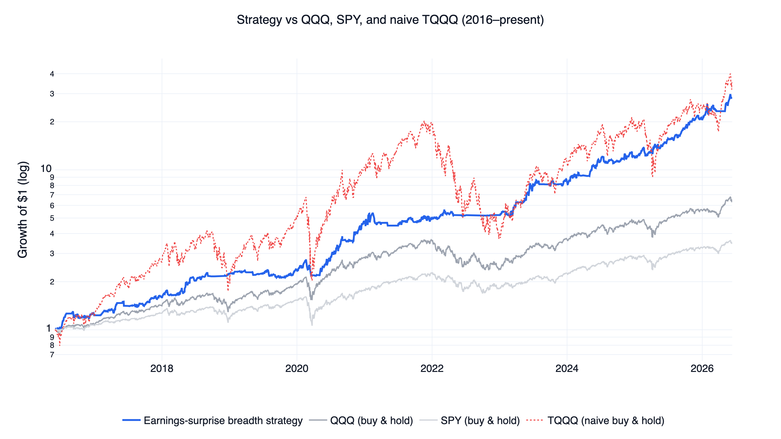
| 05 | Earnings surprise | Stock-factor breadth | 39.5% | 1.57 | -21.1% | 1.93 | 2 |
| 08 | Free cash flow | Stock-factor breadth | 37.3% | 1.53 | -21.1% | 1.95 | 2 |
| 04 | Value + quality | Stock-factor breadth | 35.9% | 1.48 | -21.1% | 1.95 | 2 |
| 03 | Quality growth | Stock-factor breadth | 33.2% | 1.39 | -21.1% | 1.95 | 2 |
| 02 | Short-term reversal | ETF timing | 67.4% | 1.43 | -27.6% | 1.50 | 1 |
| 10 | Regime risk-on/off | ETF timing | 55.1% | 1.33 | -29.3% | 1.47 | 1 |
| 07 | Breakout / trend | ETF timing | 37.2% | 1.19 | -28.3% | 1.73 | 2 |
| 09 | Sector rotation | ETF timing | 30.5% | 1.38 | -17.9% | 1.45 | 2 |
| 06 | Low volatility | ETF timing | 32.1% | 1.30 | -22.2% | 1.35 | 1 |
| — | QQQ (buy & hold) | Benchmark | 19.7% | 1.09 | -35.6% | — | 1 |
Benchmarks use total-return (dividend-adjusted) prices. The leveraged ETF series already embed each fund's daily-reset behavior and expense ratio, so the volatility drag of 2x and 3x products is in the results, not assumed away.
One execution model, ten signals
The reason this is a family and not ten coincidences is the execution layer, which is identical across every strategy. Each one answers a single question every month: is the regime supportive enough to hold leveraged growth exposure? When the answer is yes, it buys one or two leveraged ETFs (TQQQ or TECL at 3x, QLD or SSO at 2x). When the answer is no, it rotates to a single defensive ETF — treasuries, gold, or a cash-like fund. Rebalancing is monthly, with an 8% trailing stop on the leveraged leg.
What differs is only the signal that answers the question. Momentum uses the breadth of stock-level price strength; earnings surprise uses the breadth of positive earnings reactions; regime timing uses QQQ's own trend. The position you end up holding in a strong market is often the same leveraged ETF; the factor decides whether you are in it at all.
This design choice is visible in the data. The five stock-factor strategies share an identical -21.1% maximum drawdown, because they share the same stop and the same instruments — the drawdown is a property of the engine, not the factor. It is also why publishing ten near-identical posts would be misleading: the honest unit of analysis is one engine and a menu of signals.
Show Code
from finlab import data
from finlab.backtest import sim

# Two markets: single stocks drive the breadth signals; the ETFs are what you hold.
data.set_market("us")
stock_close = data.get("us_price:adj_close")     # dividend/split-adjusted

data.set_market("us_fund")
etfs = data.get("us_fund_price:adj_close")[["QQQ", "TQQQ", "TECL", "QLD", "SSO", "IEF", "GLD", "SHY"]]

# Each strategy supplies its own boolean "risk_on" series from a different factor.
# The shared part is everything after that decision:
def execute(risk_on, risk_assets, defensive="IEF"):
    position = etfs[risk_assets].where(risk_on, other=0)   # hold leverage when risk-on
    position[defensive] = (~risk_on).astype(float)          # else one defensive ETF
    return position

# Example: a QQQ-trend regime gate (strategy 10). Momentum, value, FCF, and the
# others swap in a different risk_on definition but reuse execute() unchanged.
trend = etfs["QQQ"] > etfs["QQQ"].rolling(200, min_periods=100).mean()
risk_on = trend & (etfs["QQQ"] / etfs["QQQ"].shift(126) - 1 > 0)
report = sim(execute(risk_on, ["TQQQ", "TECL"]), resample="ME", stop_loss=0.08)
Two kinds of signal: stock-factor breadth vs ETF timing
The family splits cleanly in two, and the split matters for how much validation each strategy carries.
Stock-factor breadth (strategies 01, 03, 04, 05, 08). These screen the full liquid US universe — the top 500 names by 60-day dollar volume — and measure how broad a factor is: what share of stocks are momentum leaders, or show positive earnings surprises, or combine cheap valuations with profitability. Broad participation is read as durable risk appetite, and the strategy expresses it through leveraged ETFs. Because there is a real stock universe underneath, each of these can be validated at the stock level first (decile sorts, rank information coefficients, a long-short spread) before any leverage is applied. The momentum write-up walks through that validation in full.
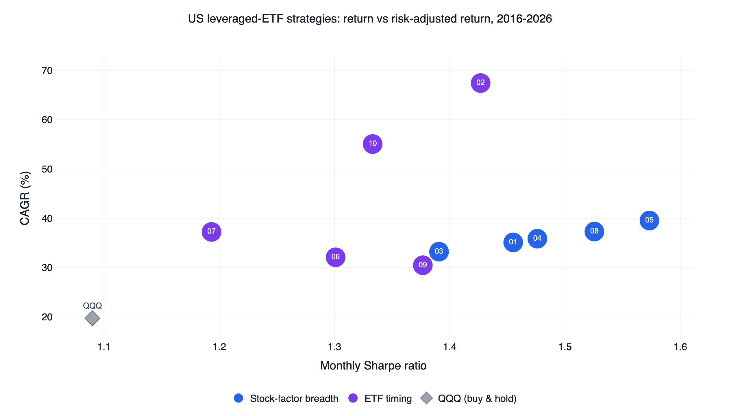
ETF timing (strategies 02, 06, 07, 09, 10). These act on the ETFs' own behavior — QQQ's trend, a breakout to new highs, short-term relative reversals between leveraged funds, or relative strength between the Nasdaq-100 and S&P 500. There is no stock universe to sort, so they cannot be validated cross-sectionally; their evidence is the time-series backtest and the economic logic of the regime rule. They tend to be more concentrated (often a single holding) and more dispersed in their results, as the scatter at the top of this page shows: the ETF-timing points span a far wider return range than the tightly clustered stock-factor group.
Risk-adjusted return: how the factors compare
Sharpe ratio is the cleaner lens than raw return, because every strategy here uses leverage and raw CAGR rewards whoever took the most risk in a bull market.
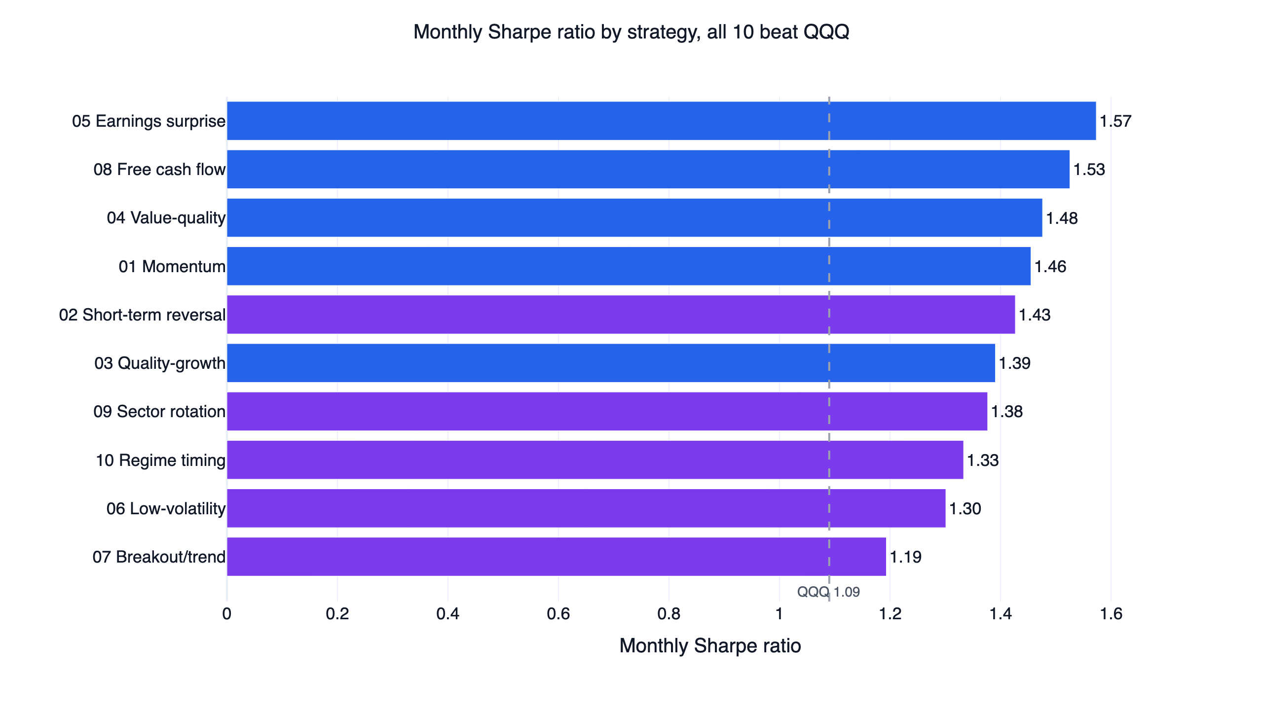
Every strategy clears QQQ's 1.09 monthly Sharpe. The stock-factor group lands in a tight 1.39 to 1.57 band, with earnings surprise (1.57), free cash flow (1.53), and value + quality (1.48) on top — fundamentals-confirmed regimes produced the steadiest risk-adjusted results. The ETF-timing group is wider: short-term reversal reaches a 1.43 Sharpe alongside the highest CAGR in the family, while breakout/trend sits at the bottom (1.19), giving up risk-adjusted quality for the chance to catch fresh highs. Higher headline CAGR did not buy a higher Sharpe; reversal and regime timing earned the two largest returns but middling Sharpes, because they also ran the largest drawdowns.
Drawdown: the shared stop shows up in the data
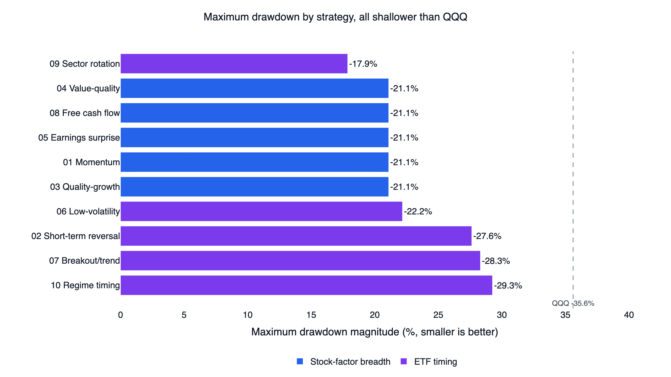
Two things stand out. First, all ten cut their worst loss below QQQ's -35.6% buy-and-hold drawdown, even while holding 2x and 3x products — the regime gate is doing real work in weak markets. Second, the five stock-factor strategies share an identical -21.1% floor. That is not a coincidence to celebrate; it is the same 8% stop on the same leveraged ETFs producing the same worst case. The ETF-timing strategies that hold a single fund and switch on faster signals (regime, breakout, reversal) ran deeper drawdowns of -27% to -29%, the price of their higher returns. Sector rotation, with the tightest stops, had the shallowest drawdown of all at -17.9% and the lowest CAGR — a direct illustration of the trade-off.
Does it survive out of sample?
Every strategy was calibrated on 2016-2021 and then left untouched on 2022-present, an unseen stretch that includes the 2022 bear market.
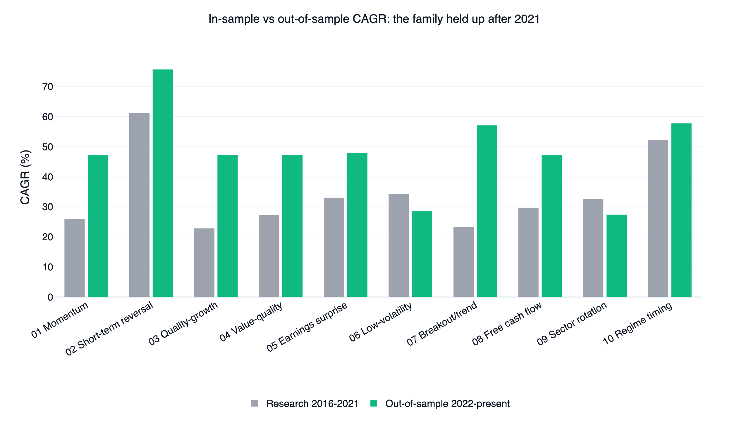
Most strategies held up or improved out of sample, with the stop-loss engine cutting risk through 2022. There is an important caveat the chart makes obvious: several stock-factor strategies post the same out-of-sample CAGR (around 47%) and Sharpe (around 1.95). That is the shared-execution design surfacing again. In a sustained risk-on regime, different breadth factors agree that conditions are supportive, so they all hold the same leveraged ETFs and their out-of-sample returns converge. Read positively, the edge is robust to which factor you pick; read skeptically, these strategies are less diversifying against each other than their names suggest, and you should not treat running several of them as genuine diversification.
Copy this prompt to your AI agent
FinLab's setup path is now one prompt. Paste it into Codex app or Claude cowork, and the AI will read https://finlab.finance/en/setup, install the FinLab skill when needed, then run or modify the strategy in this article.
Show Code
Help me set up FinLab and compare US quant trading strategies: https://finlab.finance/en/setupThe setup page is https://finlab.finance/en/setup.
The leveraged-ETF risk you must understand
Every strategy in this family holds leveraged ETFs, so they share the same core risks:
- Daily reset and path dependency. A 3x daily ETF compounds daily, so a choppy, sideways market erodes value even if the index ends flat. This is why none of these strategies hold leverage unconditionally.
- Gaps can beat stops. The 8% stop is a touched level in the backtest; a large overnight gap can fill worse in live trading.
- Monthly switching is not crash protection. A fast crash inside a month is taken at full leverage until the next rebalance.
- Concentration. Holding one or two ETFs means single-position and single-theme (large-cap US growth) risk. The higher-return ETF-timing strategies are the most concentrated.
If those risks are unacceptable to you, the stock-factor strategies can also be run unlevered on their top-decile baskets, capturing the selection edge with far less tail risk, as shown in the momentum study.
Backtest method and limits
The assumptions are shared across the family:
| Item | These backtests |
|---|---|
| Transaction costs | Not modeled (zero commission and slippage). Monthly ETF rebalancing keeps this small, but leveraged-ETF spreads and rebalance slippage would reduce live returns. |
| Leverage decay | Already reflected — the TQQQ/TECL/QLD/SSO price series include daily-reset drag and expense ratios. |
| Universe / point-in-time | Stock-factor strategies use the top 500 US names by 60-day dollar volume with price and liquidity gates; each date uses only then-available data. ETF-timing strategies trade a fixed ETF set. |
| Turnover | Roughly 2.5x to 6x per year depending on the signal — monthly regime switches, not daily churn. |
| Sample | 2016-2021 calibration; 2022-present out-of-sample. |
| Capacity | Not estimated. Leveraged ETF liquidity is large, but real impact depends on your size. |
The gate each strategy is measured against is a risk-adjusted ratio of at least 1.5. Several clear it on the full-period monthly Sharpe (earnings surprise 1.57, free cash flow 1.53), and all clear it on the 2022-present out-of-sample Sharpe; the lower full-period Sharpes (breakout 1.19, low volatility 1.30) are reported as-is rather than reframed.
Where the edge comes from
Each signal rests on a documented anomaly rather than a fitted curve. Cross-sectional momentum was established by Jegadeesh & Titman (1993) and built into a standard factor by Carhart (1997). The earnings-surprise strategy draws on post-earnings-announcement drift, documented by Bernard & Thomas (1989). The quality and free-cash-flow strategies rest on the gross-profitability premium of Novy-Marx (2013), and the low-volatility strategy on the low-beta effect formalized by Frazzini & Pedersen (2014). That momentum and value persist together across markets is the broader evidence in Asness, Moskowitz & Pedersen (2013). The contribution here is not the anomalies; it is expressing them through a disciplined leveraged-ETF regime gate and measuring the result honestly.
Read the individual strategy write-ups
Detailed studies with full validation, downloadable code, and interactive reports are published as each one is finished. Live now:
- US momentum strategy — the first full study: decile sorts, rank IC, breadth as a regime gate, and the leveraged-ETF execution in detail.
- Post-earnings announcement drift strategy — a 19,083-event earnings surprise study: why single-name PEAD barely survives in liquid large caps, and how surprise breadth still works as a regime signal.
- Quality and value strategy — three fundamental screens (quality growth, value plus quality, free cash flow) run through decile and rank-IC tests: weak as stock pickers, strong as breadth gates, and why all three converge to one trade out-of-sample.
- ETF rotation strategy — one QQQ risk-on/risk-off signal at two leverage budgets (conservative 2x, aggressive 3x): why the signal filters volatility rather than predicting returns, and what that buys for surviving leveraged-ETF compounding.
- Short-term mean reversion strategy — the family's highest CAGR (67%): a 3-day laggard rule between TQQQ and TECL inside the regime gate, with an event study showing the reversal tilt is real but statistically weak (t-stat 1.33), so the regime engine does most of the work.
- Breakout trend following strategy — fresh QQQ 21-day highs gated by a 200-day trend filter: a breakout event study where filtered highs followed through 82% of the time at three months versus 61% against the trend, and why the family's weakest full-period Sharpe (1.19) rose to 1.73 out of sample.
- Low volatility strategy — a QQQ regime filter expressed through one 2x leveraged ETF, and the most candid result in the family: naive QLD out-earned it on raw CAGR (34.8% vs 32.1%), so what the regime filter actually bought was the risk column, cutting the drawdown to -22% from -64% by forecasting volatility rather than crashes.
- New-high momentum study and the AI quant research workflow — how the breakout and research process work end to end.
- PEG value strategy, the institutional-flow strategy, and the cash-flow quality strategy — related factor research.
For definitions of the metrics used above, see the glossary. To see what teams build with finlab, browse the use cases, the research blog, and the team behind FinLab.
Who this is for
This comparison fits an investor who wants a rules-based, growth-tilted US approach, understands leveraged ETFs, and can tolerate 20%+ drawdowns in exchange for higher compounding. It does not fit anyone who needs capital stability, cannot monitor a monthly rebalance, or is uncomfortable holding 2x or 3x products at any time.
FAQ
What are these US quant trading strategies, in one sentence? Ten rules-based systems that each use a different factor to decide when to hold leveraged growth ETFs (TQQQ, TECL, QLD, SSO) and when to rotate to a defensive ETF, rebalanced monthly with an 8% stop.
Why do so many of them have similar drawdowns? Because they share the same execution: the same leveraged ETFs and the same 8% stop. The factor changes the timing, not the instrument, so the worst-case drawdown is largely a property of the engine.
Which one is "best"? There is no single best. Earnings surprise had the highest full-period Sharpe (1.57), short-term reversal the highest CAGR (67%) at a deeper drawdown, and sector rotation the shallowest drawdown (-17.9%) at the lowest CAGR. The right choice depends on how much drawdown you can hold.
Are the returns realistic given no transaction costs? Costs are not modeled. For monthly rebalancing of liquid ETFs the effect is modest, but leveraged-ETF spreads and slippage would lower live results below these figures.
Can I run and modify these myself? Yes. Use the AI-assisted setup flow and ask your agent to build any version, or download a strategy script and run it after setup.
Do I need single-stock data or just ETF data?
The stock-factor strategies need us_price:* for the screen and us_fund_price:* for the ETFs; the ETF-timing strategies need only us_fund_price:*. Both are in a standard FinLab account.
Last updated: 2026-06 | Backtest window: 2016-06 to 2026-06 | Benchmark: QQQ total return | Author: FinLab Quant Research (reviewed by a quantitative researcher)
Investing involves risk, and past performance does not represent future results. Leveraged ETFs carry additional risks including volatility decay and amplified losses. This content is for educational purposes only and is not investment advice and does not constitute investment advice; evaluate any strategy against your own risk tolerance.
FinLab AI
Want to build your own strategy?
Describe your stock-picking ideas in natural language. AI automatically validates, backtests, and gives you answers
Start Free