Algorithmic trading is the use of software to follow specified rules for investment decisions or order execution. A complete rule states what can be traded, when a signal is observed, how positions are sized and when they change. “Algo trading” can mean a monthly ETF allocation, a stock-ranking system or an execution algorithm. It does not require high-frequency trading.
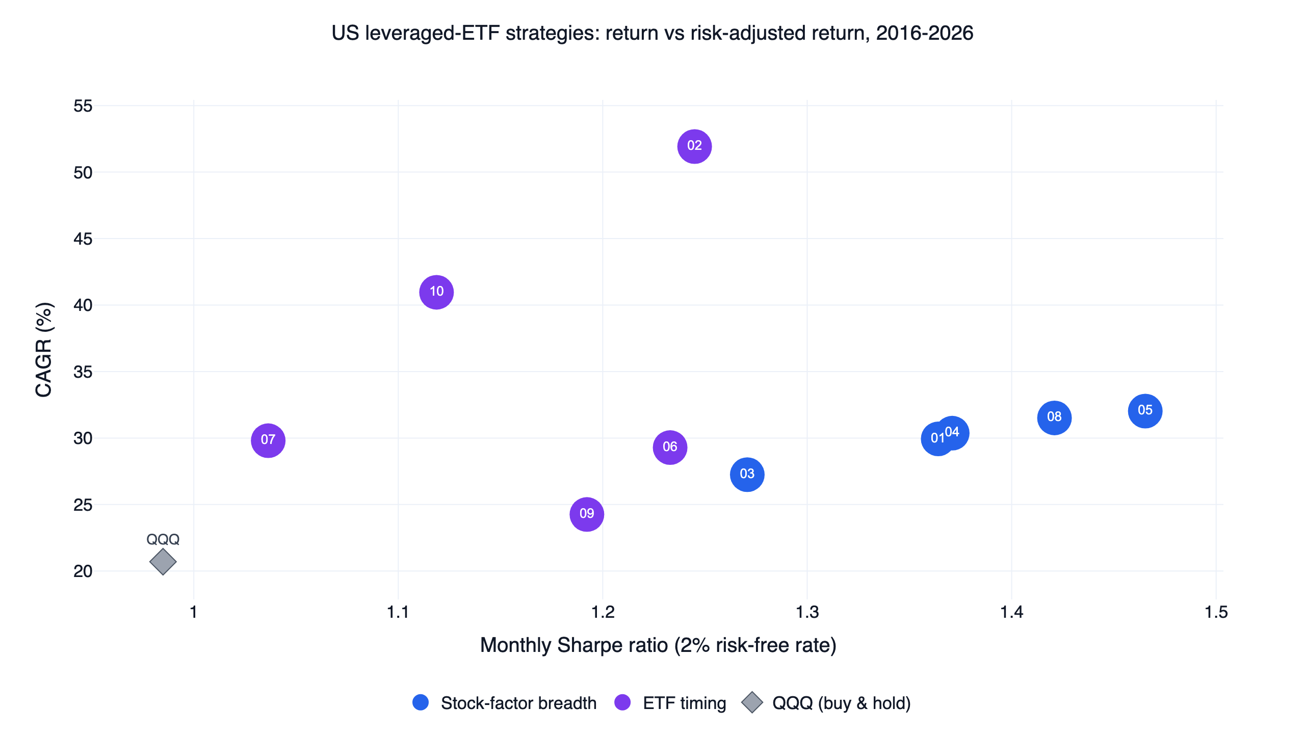
A useful first project is a reproducible research experiment. FinLab's published U.S. momentum study reports 29.9% CAGR and -21.1% maximum drawdown over May 2016 to October 2026, against QQQ at 20.7% and -35.1%. That system uses leveraged ETFs and a shared trend gate. Its result is a dated observation about a specific portfolio, not an expected return from automating any rule.
Write the specification before the code
| Decision | A specification you can test | What remains ambiguous without it |
|---|---|---|
| Universe | A fixed list of SPY and QQQ, or a dated historical stock universe | Whether current survivors were selected retroactively |
| Signal | A stated lookback and formula using information available at the decision | Which price, filing date or revised value was used |
| Timing | Observe the completed signal, then use the documented execution model | Whether the trade assumes a price already passed |
| Sizing | Fixed target weights or an explicit ranking and weight rule | Whether favorable trades received larger weights afterward |
| Rebalancing | A daily, weekly or monthly schedule | How often costs and decisions occur |
| Risk | A position limit, exit rule and treatment of cash | Whether the simulation silently exceeds intended exposure |
| Evaluation | A fixed benchmark, dates and reserved period | Whether the result was selected after seeing every period |
The specification should be readable without opening the source code. A second researcher should be able to implement the same experiment from it. If two reasonable implementations disagree about the trade date, weights or cash balance, clarify the specification before comparing their returns.
Open Studio to ask for an initial implementation, or follow the AI-assisted FinLab setup for a compatible agent on your computer. Start by asking the agent to repeat the specification and identify missing assumptions. Then ask it to run the test and return the code, report and a small trade sample.
Algorithmic trading strategies for a first U.S. study
A fixed ETF allocation tests the mechanics of weights and rebalancing. Momentum ranks past returns over a stated lookback. Mean reversion tests whether a short-term move reverses. A trend rule changes exposure when an asset crosses a defined average. A fundamental rule compares company accounts with price, aligned to public filing dates. An event rule acts after an observable announcement.
Each adds a different source of uncertainty. Price rules need corporate-action adjustments and unambiguous execution timing. Fundamental rules also need publication dates and a historical universe. Short-term rules are often more sensitive to spreads and fill assumptions. An intricate machine-learning model adds fitting decisions before any trading decision is made.
FinLab's momentum study and mean-reversion study illustrate different signal horizons. Their actual holdings are leveraged ETFs. The signal's name alone does not tell you what the portfolio owns, its leverage or its diversification. Inspect those facts in the position and trade tables.
Python for finance: a small portfolio experiment
The example below sets up an equal-weight SPY/QQQ experiment. It is a code illustration, with no performance claim. It uses the ETF market rather than the single-stock market, a monthly rebalance and an explicit cost assumption. It saves a standalone report for inspection.
Show Code
from finlab import data
from finlab.backtest import sim

# SPY and QQQ are funds, so choose the U.S. ETF/fund market.
data.set_market("us_fund")
close = data.get("us_fund_price:adj_close")[["SPY", "QQQ"]]

# Equal target weights on dates when both instruments have observations.
position = close.notna().astype(float) * 0.5
position = position.loc["2016-01-01":]

report = sim(
    position,
    resample="M",
    trade_at_price="close",
    fee_ratio=0.001,
    tax_ratio=0,
    upload=False,
)
report.to_html("spy_qqq_portfolio.html")
print(report.get_stats())
The 0.1% per-side fee is a research assumption representing friction; it is not a quote from a broker or a measured spread. Change it to fit the intended trading process, then run a higher-cost case as a sensitivity check. The example contains no predictive signal. Its purpose is to establish that the data, weighting and report work before a timing rule is introduced.
For an existing measured system, download the momentum strategy script and daily equity data from the published study. Keep the source report's dates, risk settings and benchmark when reproducing it. A new start date or a different risk-free convention creates a different experiment.
Separate data, signal, portfolio and execution
A research program is easier to inspect when each stage has a clear output. The data stage chooses adjusted prices, volumes and filings. The signal stage turns those inputs into scores or conditions. The portfolio stage converts scores into target weights. The simulation stage applies the trading schedule and costs. A live executor, if separately implemented, translates targets into orders and checks what actually filled.
This separation helps identify errors. A correct momentum score can still produce the wrong portfolio if ranking is performed down dates rather than across securities. A valid target portfolio can still produce misleading returns if a trade executes before the signal exists. An order generator can still fail operationally if it sends yesterday's targets twice.
For U.S. stocks, select data.set_market("us"); for SPY, QQQ and other funds, use us_fund. Generic data names follow the selected market. When a study mixes stock signals with ETF holdings, name the tables explicitly and verify the market again before the backtest. A stock factor can be calculated on one universe while exposure is taken through a different instrument.
Read the result before optimizing
| Published example | CAGR | Monthly Sharpe, 2% risk-free | Max drawdown |
|---|---|---|---|
| Momentum system | 29.9% | 1.36 | -21.1% |
| Earnings-surprise system | 32.0% | 1.47 | -21.1% |
| Breakout/trend system | 29.8% | 1.04 | -27.9% |
| QQQ buy and hold | 20.7% | 0.98 | -35.1% |
These same-window figures are from the U.S. strategy comparison, May 2, 2016 to October 26, 2026. The close CAGR of momentum and breakout hides a material difference in variability and drawdown. A single headline return does not tell you which implementation has stronger evidence.
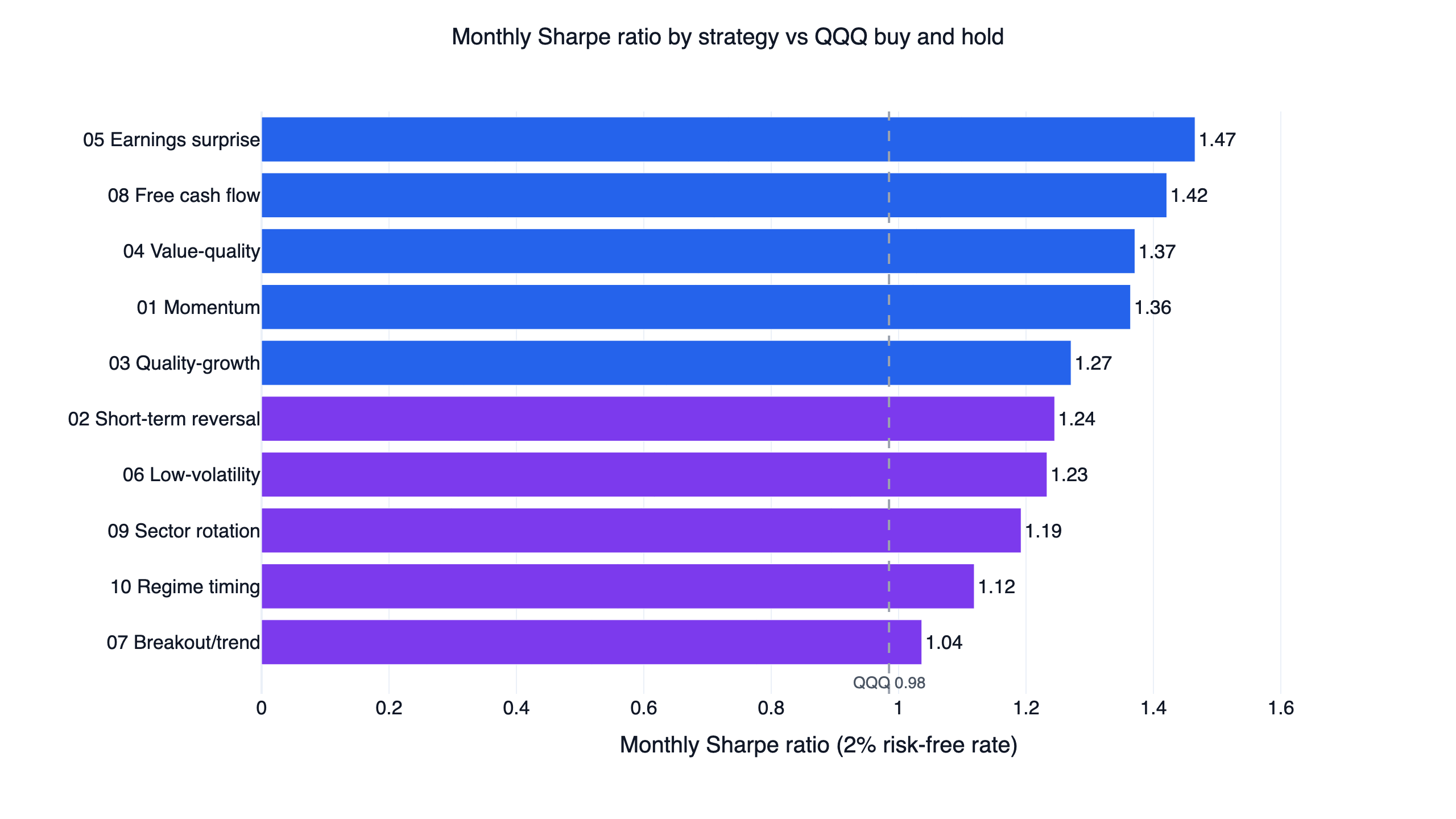
Inspect the equity curve, losing months, time in cash, number of trades and concentration. Check that buys occur after the input is available. Review one rebalance manually: starting holdings, target weights, trade amounts and costs should reconcile. If the aggregate report looks surprising, trace a few dates before adding a new filter.
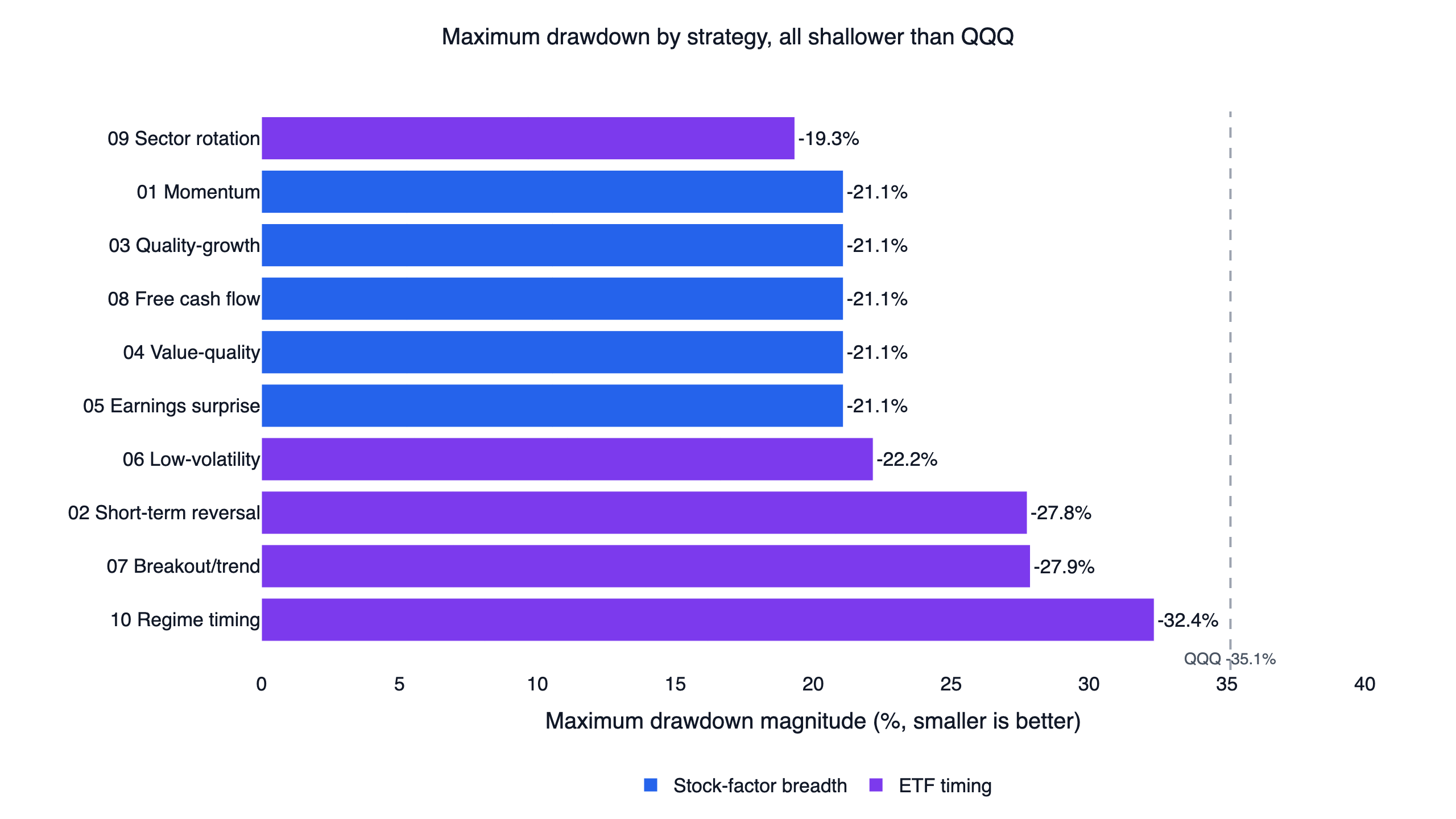
Risk rules are part of the algorithm. An 8% stop on each holding does not cap the portfolio's maximum drawdown at 8%. Repeated losses, multiple positions, overnight gaps and the assumed fill model all affect the final path. The published systems' drawdowns are measured portfolio outcomes; the stop percentage describes an instruction.
Validation that changes your decision
Reserve a period before changing parameters, compare a few neighboring settings and raise transaction costs. Ask whether the rule still offers a useful trade-off against the passive benchmark. A result that survives one test can fail another. Keep the failed result rather than changing the parameters until it disappears.
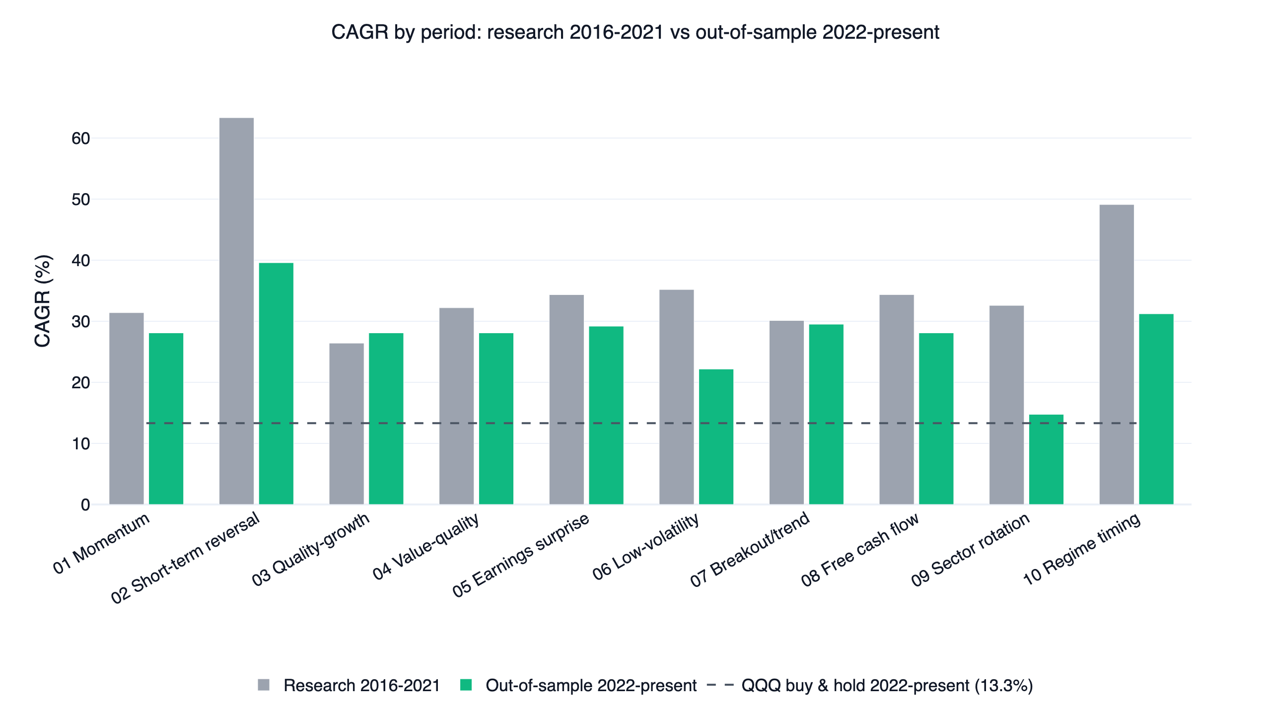
In the published comparison, breakout/trend failed the two-halves robustness test: first-half daily Sharpe was 1.16 against QQQ's 1.20. Other systems had stronger checks, but several share a QQQ gate and the same ETF holdings. Their similar outcomes therefore do not constitute independent trials of unrelated trading ideas.
Historical evaluation also has limits. A later period is useful only to the extent it was not used to design the rule. Once a researcher repeatedly inspects it and adjusts the system, it becomes part of the development process. Keep a record of what changed, why it changed and which evidence was already visible at the time.
Research automation and live execution
A completed report is the end of one experiment. A live system needs further operational work: reliable input updates, market calendars, account reconciliation, order-size limits, duplicate-order protection, fill handling and a way to stop trading. Paper trading can help examine this process, although simulated fills do not establish real execution quality.
Do not infer a brokerage connection from a natural-language prompt. An agent that writes a strategy has not necessarily obtained any account permission or sent an order. Ask it to distinguish proposed positions, simulated trades and actual orders in its output. Verify account and order details through the intended trading interface before any execution.
For a daily or monthly system, reproducibility often matters more than code speed. Save the exact script and dependencies, the data dates and the selected settings. If an input is missing, the program needs a stated policy: skip the rebalance, retain the position or stop for inspection. Decide this policy in advance rather than choosing whichever behavior improves past returns.
Frequently asked questions
Is algorithmic trading legal?
Rules depend on jurisdiction, instrument and activity. This research guide does not determine a trader's obligations. A backtest is a simulation; using a brokerage account or distributing investment services introduces separate requirements that need their own review.
Is algorithmic trading profitable?
Automation makes a rule repeatable. It does not create a return advantage by itself. The evidence comes from the rule's mechanism, its data, evaluation design, execution assumptions and subsequent results. A loss-making rule can also be automated perfectly.
Can I use ChatGPT or Claude for trading research?
A compatible agent can help with code, data inspection and reports using the FinLab skill. Studio provides a hosted research path. Ask for executed results and explicit assumptions, and verify any code or interpretation that affects the experiment.
Do I need Python to start?
You can describe a research task in Studio in English. Knowing basic Python helps you inspect the generated script and recognize a wrong column, lookback or market. Begin with a small experiment that is easy to verify rather than a large search over strategy variants.
How does this differ from quant trading?
Quant trading emphasizes research and measurement. Algorithmic trading emphasizes an explicit implementation. A useful system needs both a sound research claim and code that executes the intended rule. Passing one does not establish the other.
A repeatable research program should also record the software version and data cutoff. Those details help explain a changed result when the same script is rerun later.
Sources and next steps
The performance examples and four figures reproduce the dated U.S. comparison. The backtesting guide covers validation, while the Sharpe guide explains comparable metrics. Sharpe (1994) describes differential returns; Lo (2002) examines uncertainty in Sharpe estimates; Bailey and coauthors analyze the risk of selecting a strategy from many trials.
For education and research only. This is not investment advice. Historical performance does not guarantee future results. Leveraged ETFs have daily objectives, path-dependent returns and the potential for substantial losses.
Last updated: 2026-10. Backtest window cited: 2016-05-02 to 2026-10-26. Author: FinLab Quant Research, the team publishing reproducible stock and ETF research.