The Sharpe ratio measures average excess return per unit of return variability. It helps compare portfolios when a higher return may simply reflect more risk. Its inputs must use the same dates, frequency and risk-free convention. A Sharpe estimate describes a sample, and its uncertainty matters when comparing strategies.
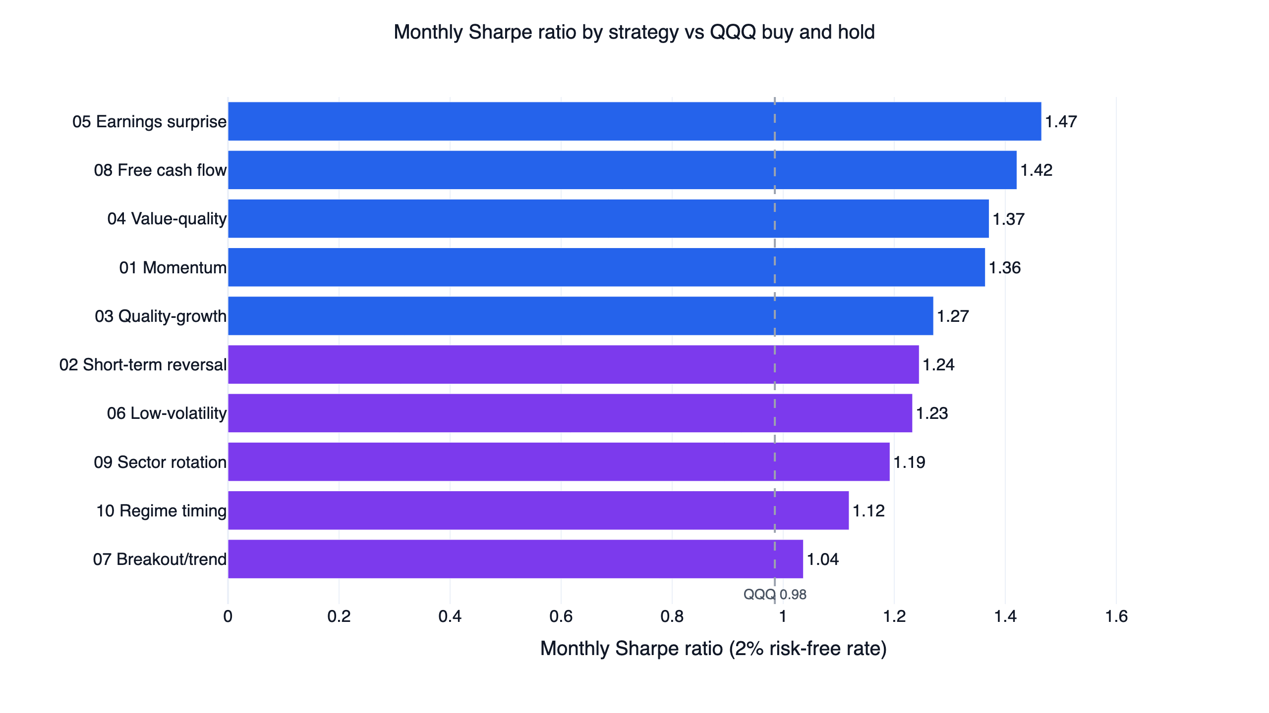
In FinLab's published U.S. comparison, the momentum system has a monthly-based annualized Sharpe of 1.36 and QQQ has 0.98, both after a 2% annual risk-free deduction over May 2, 2016 to October 26, 2026. Those numbers describe particular historical portfolios. They are not universal targets or a promise about their next decade.
Sharpe ratio formula
For regularly spaced observations, let x[t] = portfolio return[t] - risk-free return[t]. The period Sharpe is mean(x) / std(x). A common annualization multiplies this by the square root of the number of observations per year: 252 for trading-day returns or 12 for monthly returns. This scaling assumes a suitable return process; serial correlation can make the simple scaling unreliable.
When the inputs are already annualized arithmetic mean return and annualized volatility, the familiar shortcut is (annual return - annual risk-free rate) / annual volatility. All percentages need the same units. Do not put CAGR into the numerator and expect the result to match a Sharpe computed from periodic arithmetic returns.
The calculator below uses annualized summary inputs. Its initial values are illustrative inputs, not a market forecast or a measured strategy. Use the report's actual periodic return series when you need a precise reconciliation, and state the risk-free rate rather than silently assuming zero.
Sharpe ratio calculator
Adjust the inputs to compare excess return with volatility. These inputs are illustrative, not a strategy forecast.
Annualized mean return, not CAGR
Annual risk-free rate for the same currency
Annualized standard deviation of returns
Longer samples reduce estimation uncertainty
PSR uses a normal-return model. Skewness, fat tails, serial correlation, costs and multiple testing can change the inference. This calculator is educational and is not investment advice.
Open FinLab Studio to inspect the return series, Sharpe and drawdown of a U.S. stock or ETF experiment together. A complete backtest gives the portfolio path and assumptions behind the ratio.
What is a good Sharpe ratio?
There is no universal cutoff. A ratio is useful relative to a comparable benchmark, a specified sample and the uncertainty in its estimate. A short sample with one large favorable move offers different evidence from a long series spanning several market regimes. Costs, leverage, valuation smoothing and repeated strategy selection also affect interpretation.
| Observation | What it means in the measured sample | What to inspect next |
|---|---|---|
| Sharpe below zero | Mean excess return is negative | Risk-free convention, costs and weak periods |
| Sharpe above zero | Mean excess return is positive | Its size relative to noise and a passive alternative |
| Higher than a benchmark | More excess return per unit of variability on that convention | Same dates, frequency, exposure and implementation |
| Unusually high estimate | A strong historical ratio under the reported model | Data leakage, smoothing, concentration and multiple testing |
The calculator's descriptive bands are orientation labels. They are not an investment recommendation or a statistical acceptance rule. A strategy can have a higher Sharpe than QQQ and still lose money over a future period. It can also have a lower Sharpe yet serve a different portfolio objective, such as reducing exposure to a particular risk.
Compare Sharpe, Sortino, Calmar and drawdown
| Metric | Numerator | Risk denominator | Main limitation |
|---|---|---|---|
| Sharpe | Mean excess return | Standard deviation of excess returns | Treats upside and downside variability together |
| Sortino | Mean return above a chosen target | Downside deviation relative to that target | Depends on target and downside-estimation convention |
| Calmar | CAGR over a stated window | Absolute maximum drawdown in that window | Depends strongly on the worst historical path |
| Max drawdown | Not a return ratio | Deepest decline from a previous equity peak | Does not state how often or how long losses occurred |
Sortino focuses on returns below a stated minimum acceptable return. A common downside-deviation convention takes the square root of the mean squared shortfall below that target, including zero shortfalls for observations above it. Other implementations condition only on downside observations. These are different conventions, so record the target and implementation before comparing published numbers.
Calmar is commonly CAGR / abs(max drawdown) for the same window. A zero drawdown makes the denominator unsuitable; a short, favorable sample can make the ratio appear extreme. Calmar uses the single worst decline, whereas Sharpe uses the distribution of periodic returns. Neither captures every feature of the investment experience.
Maximum drawdown at a date is the equity value divided by the highest earlier equity value, minus one. The maximum drawdown of the sample is the most negative of these observations. A -25% drawdown needs a 33.3% gain to recover the prior peak, because the recovery starts from a smaller base. This is arithmetic about a loss, not a strategy forecast.
Max drawdown calculator
Paste a regularly sampled equity series or periodic percentage returns. The calculator uses those observations only, so a monthly series may miss deeper losses between month ends. Choose periods per year to match your data. The initial sequence is an illustration; replace it with your own report values for a portfolio calculation.
Max drawdown and CAGR calculator
Paste regularly spaced equity values or returns to calculate maximum drawdown and CAGR. Calculations stay in your browser.
Paste account values sampled at regular intervals
Read 7 valid numbers. The initial series is illustrative and is not a real strategy result.
Use 252 for daily trading data, 12 for monthly data or 52 for weekly data. Choose the frequency of your own observations.
Drawdown measures the largest loss from a peak. CAGR describes compounded growth. Read both alongside Sharpe. This calculator is not investment advice. Explore the quant tools for more context.
Do not infer a future loss limit from historical maximum drawdown. A new market event can exceed it. Inspect the duration of declines and recovery as well as depth, especially when comparing leveraged portfolios or portfolios that remain in cash for extended periods.
U.S. examples: a return ranking differs from a risk ranking
These same-window results reproduce the U.S. strategy comparison, May 2016 to October 2026. Sharpe is annualized from monthly returns with a 2% annual risk-free deduction. QQQ and SPY are dividend-adjusted buy-and-hold benchmarks.
| System | CAGR | Monthly Sharpe (2% risk-free) | Max drawdown |
|---|---|---|---|
| Earnings surprise | 32.0% | 1.47 | -21.1% |
| Momentum | 29.9% | 1.36 | -21.1% |
| Mean reversion | 51.9% | 1.24 | -27.8% |
| Conservative ETF rotation | 24.3% | 1.19 | -19.3% |
| QQQ | 20.7% | 0.98 | -35.1% |
| SPY | 15.1% | 0.88 | -33.7% |
The mean-reversion system has a higher CAGR than earnings surprise but a lower Sharpe and deeper drawdown. Conservative rotation has the lowest strategy CAGR in this selection, paired with the shallowest drawdown. Read these as distinct historical trade-offs. The strategies use 2x or 3x ETFs and different portfolio structures; the labels alone do not reveal the actual risk taken.
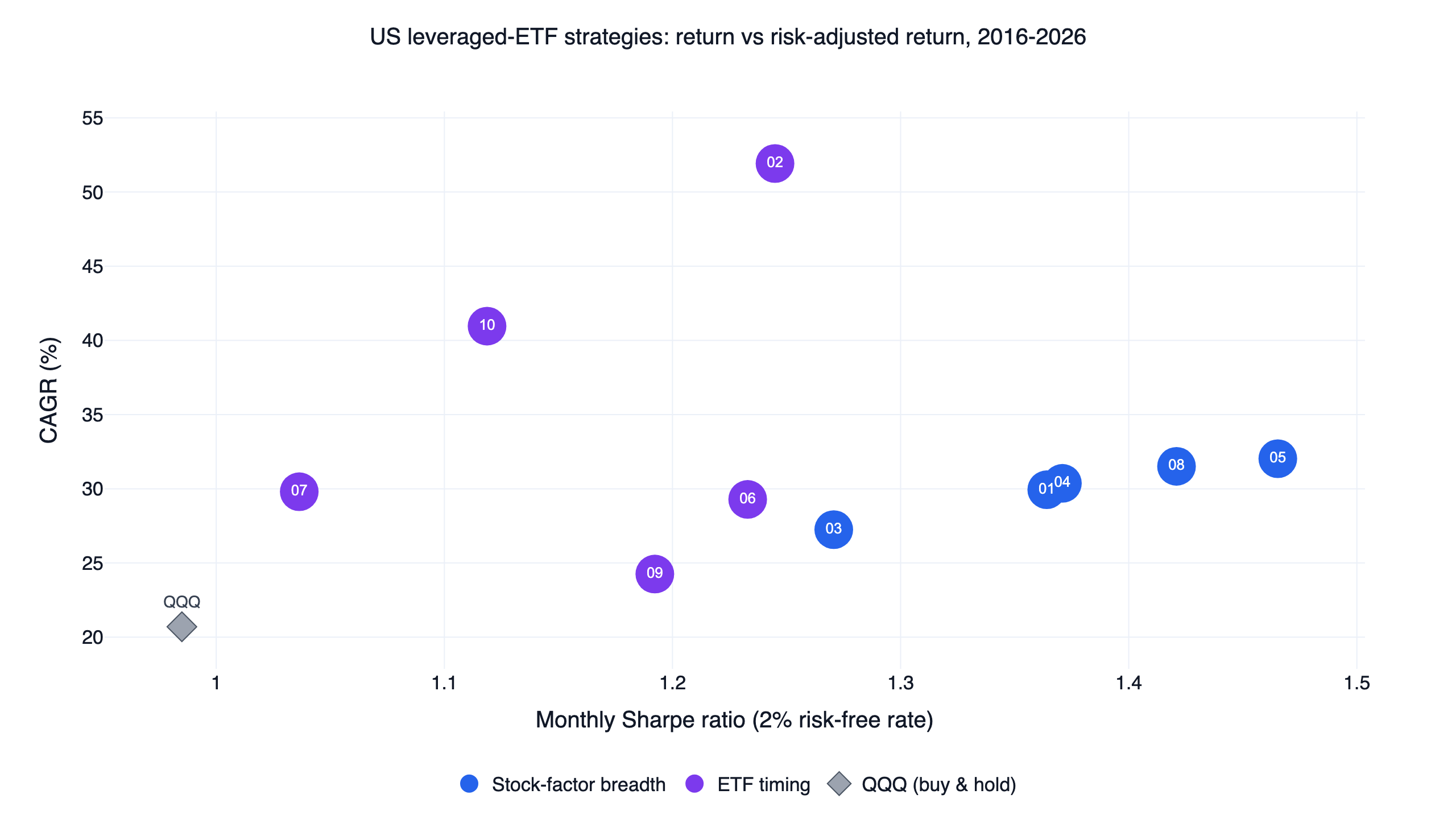
The scatter places the systems in return-risk space. Taking more exposure can increase both return and volatility. A higher raw return therefore needs an explanation of leverage, cash holdings and concentration before it becomes evidence of better investment selection.
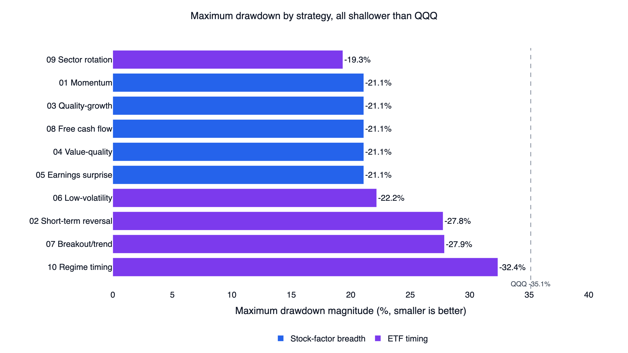
Several stock-factor systems share the same -21.1% drawdown because they share an execution model and holdings. Those repetitions should not be counted as independent confirmations of a low-risk signal. Inspect overlapping positions when using multiple strategies in a portfolio.
Why your Sharpe may differ from a published report
A daily Sharpe and a monthly Sharpe can differ because aggregation changes the observed return distribution. A zero-risk-free estimate differs from one with a positive deduction. Arithmetic mean return differs from CAGR. An equity series including cash flows can differ from a time-weighted return series. Missing observations and sample-standard-deviation choices can matter as well.
The momentum study illustrates the convention issue directly: its full-window monthly Sharpe without a risk-free deduction is 1.46, while the shared comparison deducts 2% and reports 1.36. The underlying system has not become a different strategy. Compare the denominator, frequency and risk-free treatment before treating a small difference as an error or improvement.
Single-stock pages provide another convenient source of context. Inspect the stated statistics on the English SPY and QQQ pages, then read their displayed windows before comparing with a research report. A current stock-page snapshot and a fixed historical experiment need not cover the same dates.
Calculate Sharpe from a saved equity curve
This example uses a completed report's equity curve and a stated zero risk-free rate. It produces a daily-based estimate; do not expect it to equal a monthly report statistic with a different deduction.
Show Code
import numpy as np

returns = report.daily_creturn.pct_change().dropna()
risk_free_per_day = 0.0
excess = returns - risk_free_per_day
volatility = excess.std(ddof=1)
sharpe = excess.mean() / volatility * np.sqrt(252)
print(f"Daily-based annualized Sharpe: {sharpe:.2f}")
The expression requires a nonzero sample volatility and a regularly sampled series. Check those inputs before using the number. Save the original report so the calendar, cash treatment and return history remain available for inspection.
Estimation risk and out-of-sample checks
An estimated Sharpe can look high by chance. Normal-return models simplify inference, but real returns may have serial correlation, skewness and heavy tails. Trying many rules and publishing only the winner adds selection bias. A calculator using one set of summary inputs cannot account for an undisclosed strategy search.
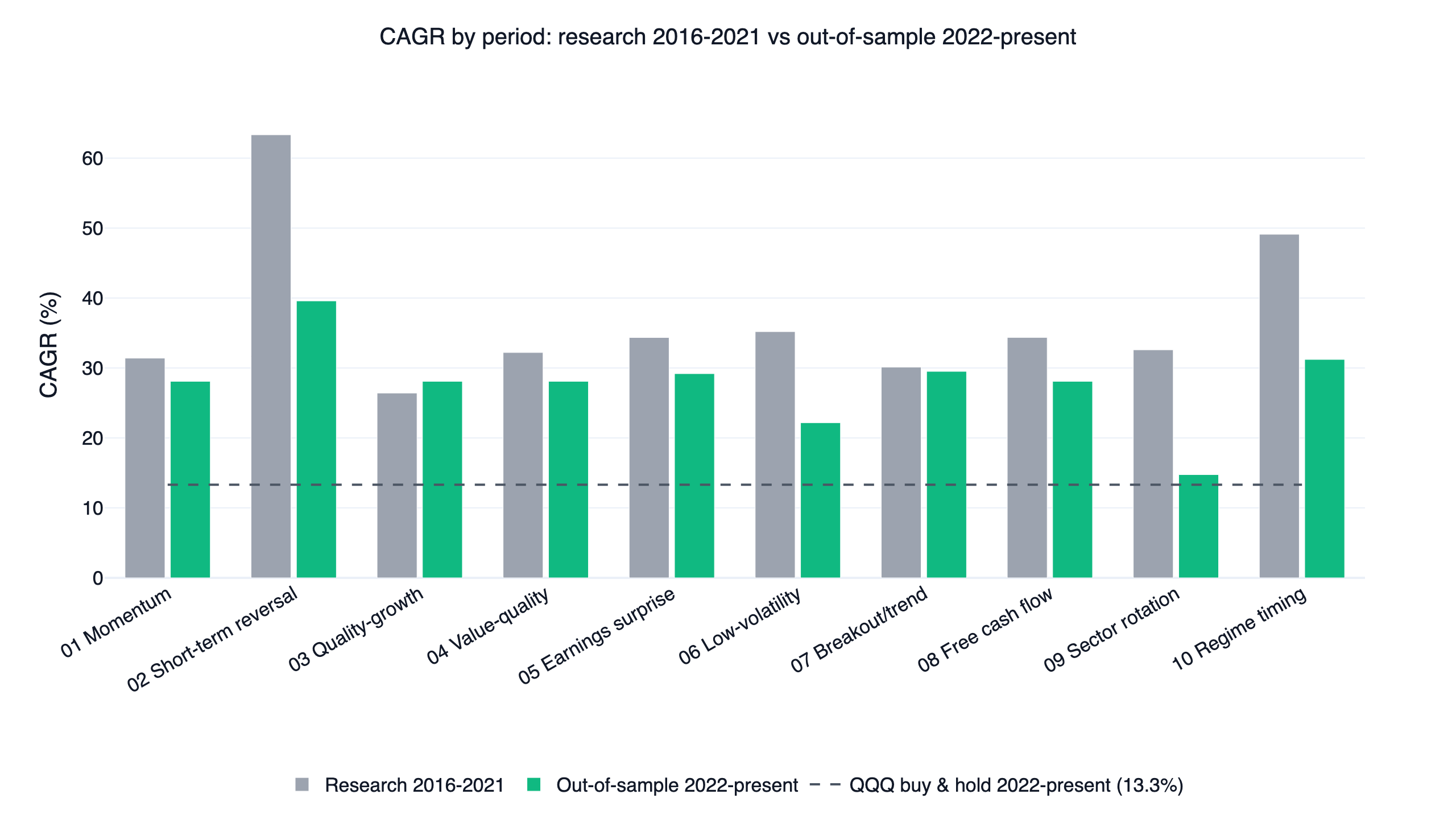
The research collection separates 2016–2021 from 2022 onward. It also checks nearby parameters, two halves of the full sample and a higher trading-cost assumption. Breakout/trend failed the two-halves comparison, even though its full-window monthly Sharpe exceeded QQQ's. A full-period ratio can conceal that dependence on a favorable subperiod.
Use look-ahead checks, cost sensitivity and a frozen evaluation rule before interpreting a small Sharpe advantage. Compare the strategy with a simpler portfolio and ask which practical decision the ratio changes. A numerical difference can be statistically uncertain and economically too small to justify extra turnover or complexity.
Frequently asked questions
Does Sharpe use total return or excess return?
The conventional calculation uses periodic returns above a risk-free return. Total-return prices are useful for measuring the portfolio's return before subtracting that reference. State both the dividend treatment and risk-free convention so the inputs can be reproduced.
Can a Sharpe ratio be negative?
Yes. If average excess return is negative and variability is positive, the ratio is negative. Rankings among negative values need care because changing volatility can change the ratio in unintuitive ways. Read the return and loss path alongside it.
Is Sortino always better than Sharpe?
It answers a different question by emphasizing downside relative to a target. That focus can be useful, but the target and convention introduce choices. Inspect both rather than selecting whichever ratio makes the strategy look stronger.
Can I use a Sharpe calculator to choose a stock?
A calculator measures an input series or supplied summary values. It does not assess the complete business, valuation, concentration or future distribution. Use it as one part of a documented research process, with a benchmark and CAGR and drawdown context.
How do I reproduce the published risk metrics?
Use the source study's script, dates and equity data. Match its frequency and risk-free assumptions before comparing. The algorithmic trading guide explains the program structure, and the quant trading guide links the research families.
Sources and research notes
Sharpe (1994) defines differential-return measurement. Lo (2002) studies the statistical properties of Sharpe estimates. Bailey and coauthors examine backtest selection and overfitting. The numerical examples and figures on this page come from the dated FinLab U.S. comparison, not from a new optimization.
For education and research only. This is not investment advice. Historical performance does not guarantee future results. Leveraged ETFs reset daily, introduce path dependence and can suffer substantial losses.
Last updated: 2026-10. Backtest window cited: 2016-05-02 to 2026-10-26. Author: FinLab Quant Research, the team publishing reproducible stock and ETF strategy studies.