Run this strategy
Copy the prompt to reproduce the evidence above with the article’s data, assumptions, and risk checks.
Tell your AI:
Set up FinLab and backtest an equal risk contribution portfolio of QQQ, TLT and GLD with a 10-month trend filter against QQQ, with and without deducting T-bills. Please read: https://finlab.finance/en/setup?relatedUrl=/en/blog/risk-parity-portfolio-backtest
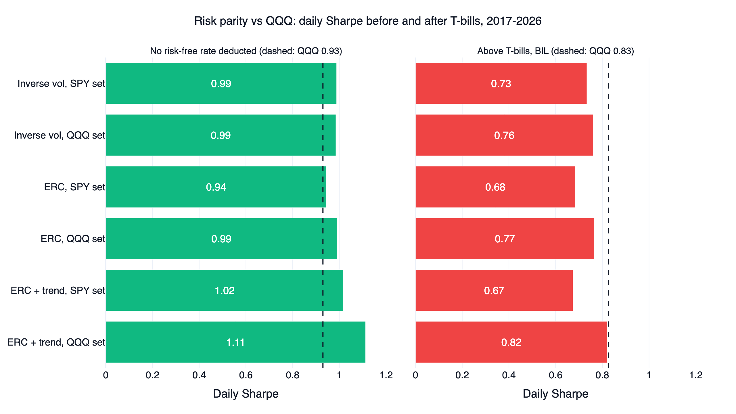
A risk parity portfolio sizes each asset by the risk it adds, so low-volatility bonds get more capital than stocks. We backtested six unlevered versions on US ETFs from January 2017 to October 2026: inverse volatility, equal risk contribution (ERC) and ERC with a trend filter, each on SPY, TLT, GLD, DBC and on QQQ, TLT, GLD. On plain daily Sharpe, 51 of the 54 settings beat QQQ's 0.93. With the T-bill return deducted, 0 of 54 beat QQQ's 0.83. None of the six designs passed our checks, so none became a strategy page.
The closest was ERC plus a 10-month trend filter on QQQ, TLT and GLD: daily Sharpe 1.11, 9.0% a year and a -13.0% maximum drawdown, against 0.93, 20.4% and -35.1% for QQQ. Above T-bills it scored 0.82 against 0.83, and it lost the first half on both measures. The two listed funds trailed 60/40 as well as QQQ: RPAR returned 3.6% a year since December 2019 and UPAR -2.1% a year since January 2022.
Key numbers
| Portfolio | Daily Sharpe | Above T-bills | CAGR | Max drawdown | Settings beating QQQ: no risk-free rate / above T-bills | Result |
|---|---|---|---|---|---|---|
| Inverse volatility, SPY set | 0.99 | 0.73 | 9.1% | -20.5% | 8/9, 0/9 | Fails |
| Inverse volatility, QQQ set | 0.99 | 0.76 | 10.2% | -25.1% | 9/9, 0/9 | Fails |
| ERC, SPY set | 0.94 | 0.68 | 8.4% | -20.8% | 7/9, 0/9 | Fails |
| ERC, QQQ set | 0.99 | 0.77 | 10.3% | -25.9% | 9/9, 0/9 | Fails |
| ERC + trend, SPY set | 1.02 | 0.67 | 6.9% | -9.0% | 9/9, 0/9 | Fails |
| ERC + trend, QQQ set | 1.11 | 0.82 | 9.0% | -13.0% | 9/9, 0/9 | Fails |
| Equal weights, SPY set (control) | 1.02 | 0.78 | 9.9% | -18.4% | ||
| Equal weights, QQQ set (control) | 0.99 | 0.79 | 11.2% | -27.1% | ||
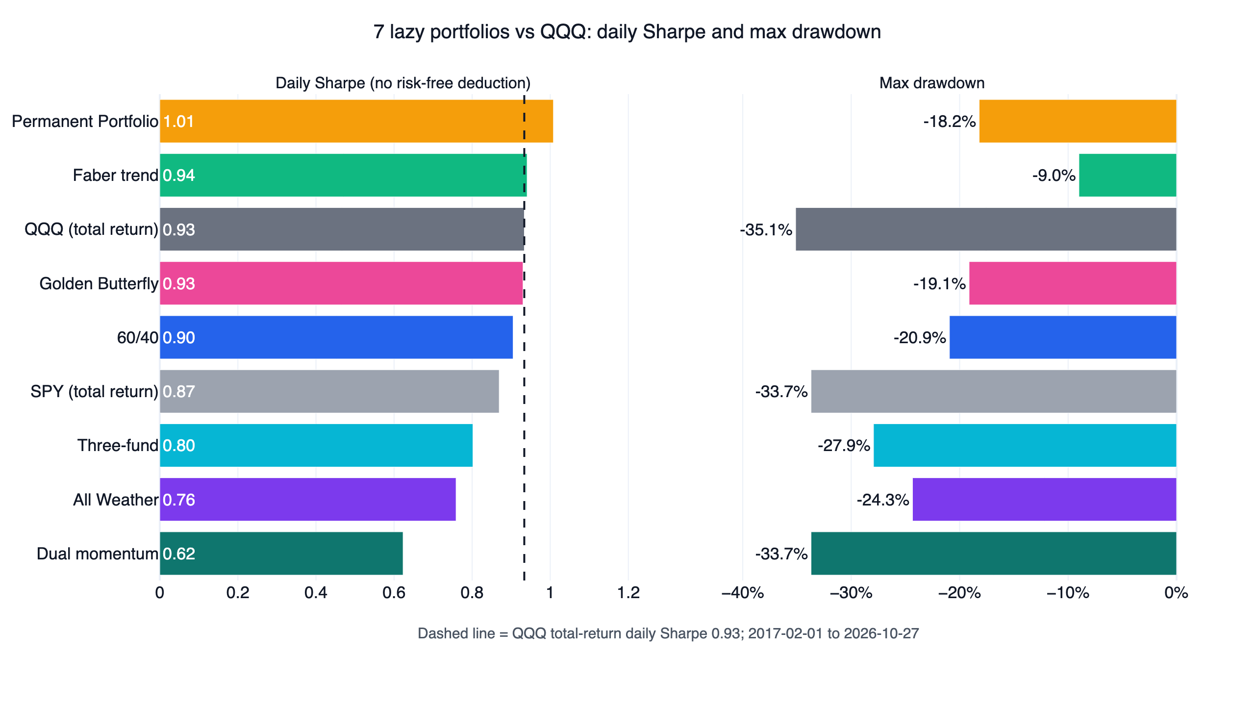
| Permanent Portfolio (control) | 1.00 | 0.69 | 7.7% | -18.2% | ||
| 60/40, SPY and AGG (control) | 0.90 | 0.69 | 9.9% | -20.9% | ||
| All Weather, simplified (control) | 0.75 | 0.49 | 6.5% | -24.3% | ||
| QQQ buy and hold, dividends reinvested | 0.93 | 0.83 | 20.4% | -35.1% | benchmark |
The SPY set is SPY, TLT, GLD and DBC; the QQQ set is QQQ, TLT and GLD. All rows use the same days, from the first fill on 2017-01-03 to 2026-10-30. The designs are unlevered and backtested at finlab's default zero cost. The three controls from our lazy portfolio backtest keep that study's quarterly rebalancing and the same ETFs, on this window.
What risk parity is
A dollar in stocks and a dollar in Treasuries do not carry the same risk. Risk parity starts from that and asks how much capital each asset should get so that each one moves the portfolio by a similar amount. The result holds more of the calmer assets and less of the volatile ones. There are two common ways to compute it.
- Inverse volatility. Each weight is proportional to one over the asset's recent volatility. It is one line of arithmetic and it ignores correlations.
- Equal risk contribution. Maillard, Roncalli & Teiletche (2010) define a portfolio where every asset's weight times its marginal contribution to portfolio risk comes out equal. That takes the full covariance matrix and a solver; we use the cyclical coordinate descent of Griveau-Billion, Richard & Roncalli (2013).
Correlations are what separate the two. This table shows the average capital weight and the average share of portfolio variance at each month end, using the trailing 63-day covariance.
| Asset | Inverse vol: capital | Inverse vol: risk | ERC: capital | ERC: risk |
|---|---|---|---|---|
| SPY | 26% | 23% | 27% | 25% |
| TLT | 27% | 20% | 31% | 25% |
| GLD | 25% | 32% | 21% | 25% |
| DBC | 22% | 26% | 21% | 25% |
| QQQ (QQQ set) | 26% | 27% | 29% | 33% |
| TLT (QQQ set) | 38% | 34% | 38% | 33% |
| GLD (QQQ set) | 35% | 38% | 33% | 33% |
Inverse volatility gives every asset the same standalone risk, but an asset that moves with the rest of the portfolio adds more. Over this window gold's daily returns correlated positively with SPY, TLT and DBC, while TLT correlated negatively with SPY and DBC. So gold ended up with nearly a third of the SPY set's risk and TLT with a fifth. ERC moved capital from gold to Treasuries until the shares matched.
The usual argument for risk parity comes from Asness, Frazzini & Pedersen (2012): investors who cannot or will not borrow overpay for risky assets, so safer assets earn more per unit of risk. Their US risk parity portfolio, scaled to the volatility of a value-weighted US stock and bond portfolio, beat that portfolio by about 4% a year from 1926 to 2010. That result relies on leverage, which matters below.
Ray Dalio's All Weather is the best-known relative, and the version most retail investors see holds fixed weights: 30% stocks, 55% Treasuries, 7.5% each in gold and commodities. The designs here recompute their weights from recent volatility. The fixed version is covered in the lazy portfolio backtest.
How a design had to pass
We fixed the six designs, their grids and the pass rules before running anything, and nothing changed after we saw results.
"Beats QQQ" here is stricter than on most of this site. A design has to post a higher daily Sharpe ratio than QQQ with dividends reinvested on the same dates, both with no risk-free rate deducted and on returns above T-bills (BIL). The second measure is there because the first flatters bonds and cash: over this window BIL held alone scored a daily Sharpe of 9.35, simply because its return barely moves. Three checks then apply.
- Neighbouring parameters. A 3x3 grid of two parameters around the original setting, nine settings, at least seven must win. Inverse volatility and ERC use a 21, 63 or 126-day window with rebalancing every 1, 2 or 3 months (original: 63 days, monthly). The trend designs use an 8, 10 or 12-month average with a 21, 63 or 126-day window, rebalanced monthly (original: 10 months, 63 days).
- Both halves. Split at the midpoint, 2021-11-29. The original setting must win each half.
- Costs. finlab's default for US funds is zero. The original setting must win at that cost and at 0.1% per side.
A combination also has to earn its keep: each trend design must beat, at its original setting, both the same ERC weights without the filter and the same filter on equal weights.
| Design | Neighbours above T-bills | First half (QQQ 1.25 / 1.21) | Second half (QQQ 0.62 / 0.46) | 0.1% per side (QQQ 0.93 / 0.83) |
|---|---|---|---|---|
| Inverse volatility, SPY set | 0/9 | 1.22 / 1.10 | 0.81 / 0.44 | 0.98 / 0.72 |
| Inverse volatility, QQQ set | 0/9 | 1.39 / 1.29 | 0.67 / 0.34 | 0.98 / 0.75 |
| ERC, SPY set | 0/9 | 1.24 / 1.12 | 0.71 / 0.33 | 0.93 / 0.67 |
| ERC, QQQ set | 0/9 | 1.45 / 1.34 | 0.63 / 0.31 | 0.98 / 0.76 |
| ERC + trend, SPY set | 0/9 | 1.13 / 0.99 | 0.91 / 0.37 | 0.95 / 0.61 |
| ERC + trend, QQQ set | 0/9 | 1.19 / 1.07 | 1.03 / 0.57 | 1.06 / 0.77 |
Each pair is daily Sharpe with no risk-free rate, then above T-bills. Had the plain Sharpe been the only test, inverse volatility and ERC on the QQQ set would have passed all three checks: nine of nine neighbours, both halves, and 0.98 against 0.93 after costs. The T-bill measure is what stopped them.
Result 1: 51 of 54 settings win until T-bills come out
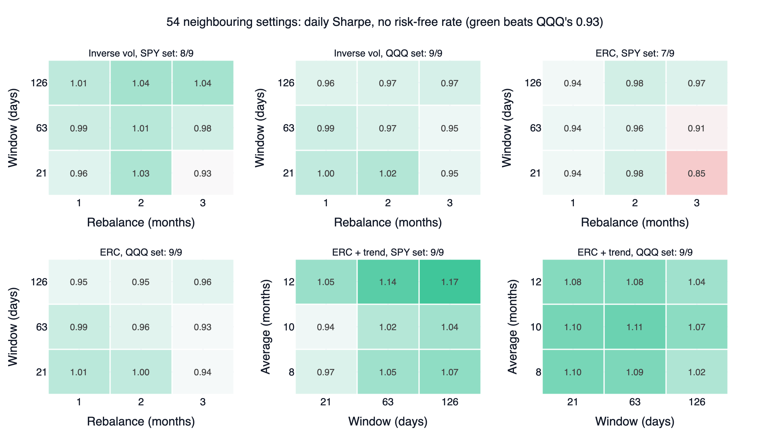
With no risk-free rate deducted, the grids are almost entirely green. Every design clears the seven-of-nine bar, and the only three losing cells are 21-day inverse volatility on the SPY set at a three-month rebalance (0.93, just under QQQ) and two ERC cells on the same set.
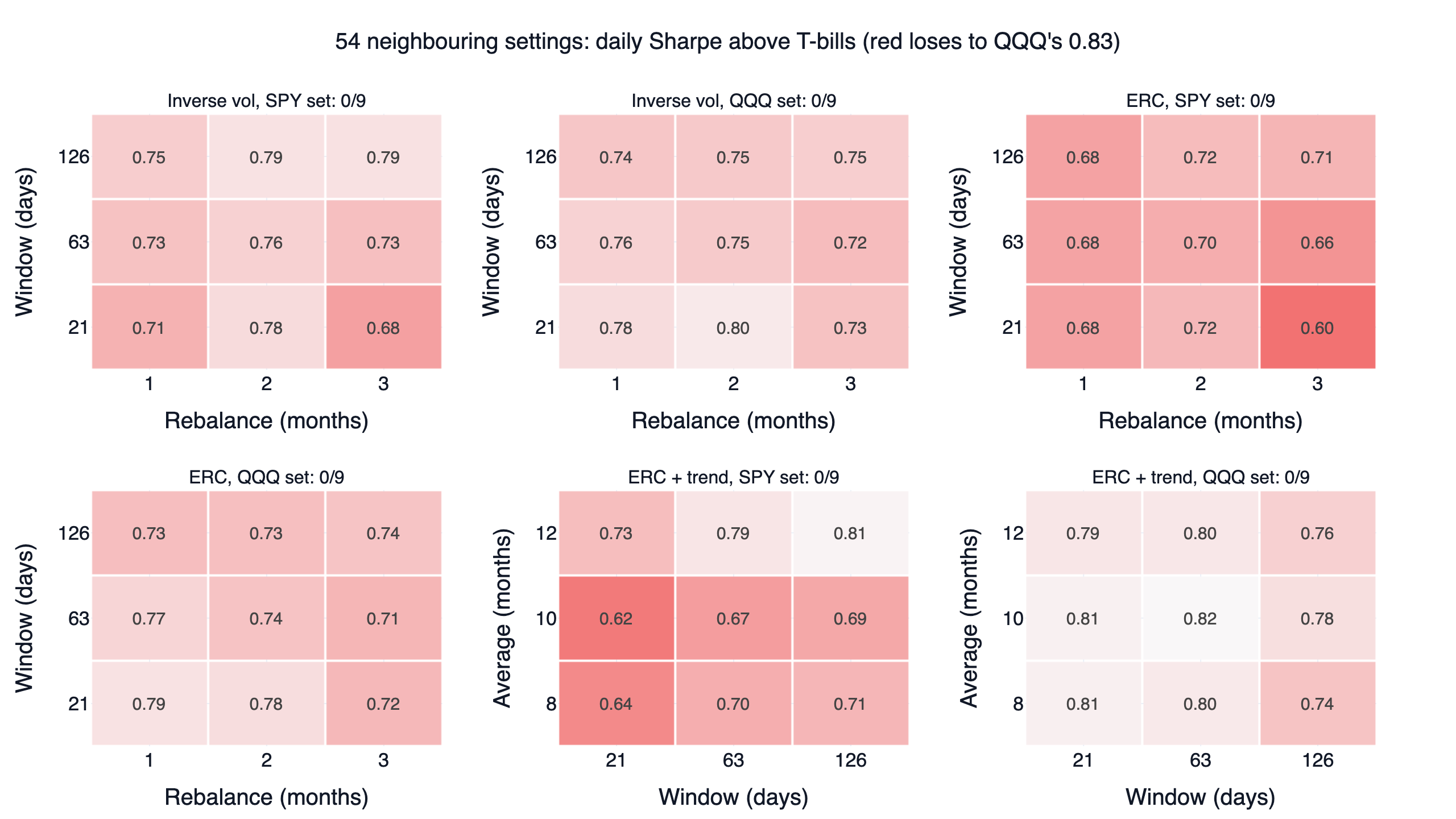
Above T-bills, every cell loses. The best of the 54 is the original ERC + trend setting on the QQQ set at 0.82; the worst is 0.60. Nothing about the designs changed between the two pictures. T-bills returned 2.4% a year here, and that return counts for more in a calmer portfolio. Divide 2.4% by ERC's 10.4% volatility and you get 0.23 of Sharpe. Divide it by QQQ's 22.8% and you get about 0.10. The actual drops match: ERC on the QQQ set falls from 0.99 to 0.77 and QQQ from 0.93 to 0.83, so a lead of 0.06 turns into a deficit of 0.06.
For risk parity the second number is the fair one, because the idea depends on leverage. Taking ERC to QQQ's level of risk means borrowing, and borrowing costs at least the T-bill rate. The Sharpe above T-bills is the part that survives. This table levers each design to QQQ's 22.8% volatility, paying only the BIL return on the loan.
| Design at QQQ's volatility | Leverage | CAGR | Max drawdown |
|---|---|---|---|
| ERC + trend, QQQ set | 2.83x | 20.2% | -33.4% |
| ERC, QQQ set | 2.18x | 18.7% | -49.5% |
| Inverse volatility, QQQ set | 2.17x | 18.6% | -48.2% |
| Inverse volatility, SPY set | 2.47x | 17.8% | -44.9% |
| ERC, SPY set | 2.53x | 16.5% | -46.4% |
| ERC + trend, SPY set | 3.34x | 16.2% | -37.6% |
| QQQ, no leverage | 1x | 20.4% | -35.1% |
At the same volatility all six earned less than QQQ. Only ERC + trend on the QQQ set drew down less, and it came within 0.2 points of QQQ's return. The calculation is generous: leverage is constant and picked with hindsight to match QQQ, and there are no margin spreads or futures costs.
Result 2: sizing by risk did not beat equal weights
| Assets and measure | Equal weights | Inverse volatility | ERC |
|---|---|---|---|
| SPY set, no risk-free rate | 1.02 | 0.99 | 0.94 |
| SPY set, above T-bills | 0.78 | 0.73 | 0.68 |
| QQQ set, no risk-free rate | 0.99 | 0.99 | 0.99 |
| QQQ set, above T-bills | 0.79 | 0.76 | 0.77 |
The simplest split matched or beat both risk-based weightings on every line. DeMiguel, Garlappi & Uppal (2009) found one-over-N hard to beat among mean-variance portfolios because of estimation error. Risk weighting estimates no expected returns, so the cause here is different.
Part of the reason is plain. Risk weighting moves capital toward the lowest-volatility asset, which was TLT. TLT lost 1.0% a year while gold made 12.7% and commodities 10.0%. ERC held TLT at an average of 31% in the SPY set and 38% in the QQQ set, against 25% and 33% under equal weights, so the extra capital went to the one asset that lost money. Holding ERC's average weights fixed explains about half of the SPY-set shortfall (0.99 and 0.73); the rest came from how the weights moved. On the QQQ set the moving weights helped: 0.99 and 0.77 against 0.93 and 0.72 for the fixed average.
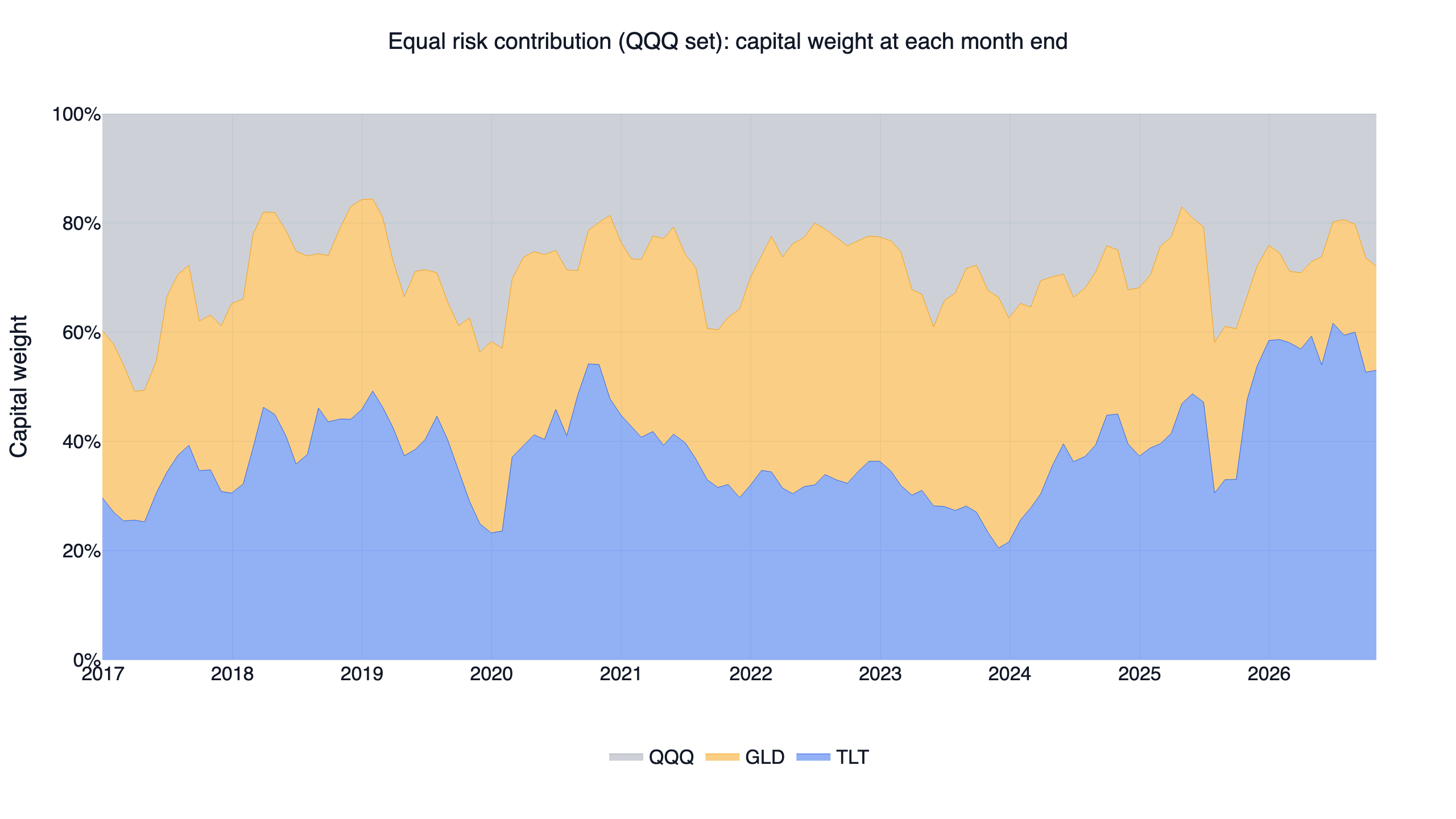
TLT's weight in the QQQ set moved between 20% and 62%, and it stood at 53% at the end of October 2026, when its 63-day volatility of 10.8% was the lowest of the three (QQQ 18.8%, GLD 24.7%).
Sizing by risk still did better than the fixed retail mix. ERC on the SPY set holds the same four asset classes as simplified All Weather and scored 0.94 and 0.68 against All Weather's 0.75 and 0.49. All Weather keeps 55% in Treasuries whatever happens; ERC averaged 31%.
Result 3: the trend filter added the most and still fell short
| QQQ set | Daily Sharpe | Above T-bills | CAGR | Max drawdown | 2022 |
|---|---|---|---|---|---|
| ERC alone | 0.99 | 0.77 | 10.3% | -25.9% | -20.2% |
| 10-month filter on equal weights | 1.08 | 0.81 | 9.4% | -13.0% | -4.4% |
| ERC + 10-month filter | 1.11 | 0.82 | 9.0% | -13.0% | -4.5% |
| QQQ | 0.93 | 0.83 | 20.4% | -35.1% | -32.6% |
The filter comes from Faber (2007): at each month end, an asset at or below its 10-month average gives its slice to T-bills. On the QQQ set the combination beat both of its parts, cut the worst drawdown by half and took 2022 from -20.2% to -4.5%. It was fully in T-bills at 10 of 119 month ends: October and November 2018, January 2022 and May to November 2022.
It still failed. Unrounded, the 0.82 is 0.821 against QQQ's 0.827, it lost the first half (1.19 against 1.25, and 1.07 against 1.21 above T-bills), and it trades about 2.25 times the portfolio a year, so 0.1% per side takes it to 0.77 above T-bills. It also sat 34% in T-bills on average, the kind of portfolio the plain Sharpe favours most.
A control sharpens the point. Holding this design's average weights fixed (25% QQQ, 18% TLT, 23% GLD, 34% BIL) scored 1.15 and 0.85 with a -18.3% drawdown. Those weights are known only with hindsight, so this is no strategy, and it lost the second half above T-bills, 0.41 against 0.46. On the plain Sharpe, part of that score is the T-bill slice itself. Above T-bills the slice adds nothing, and the fixed mix still scored higher, 0.85 against 0.82. In this window the monthly filter added no Sharpe over a static mix; what it added was the shallower drawdown, -13.0% against -18.3%.
On the SPY set the combination failed its extra test: ERC + trend scored 1.02 and 0.67 against 1.05 and 0.72 for the same filter on equal weights, and above T-bills the filter left ERC slightly lower, 0.67 against 0.68. The 12-month row of its heatmap looks better (1.05 to 1.17), but the original setting was fixed in advance, and the best cell still lost above T-bills at 0.81.
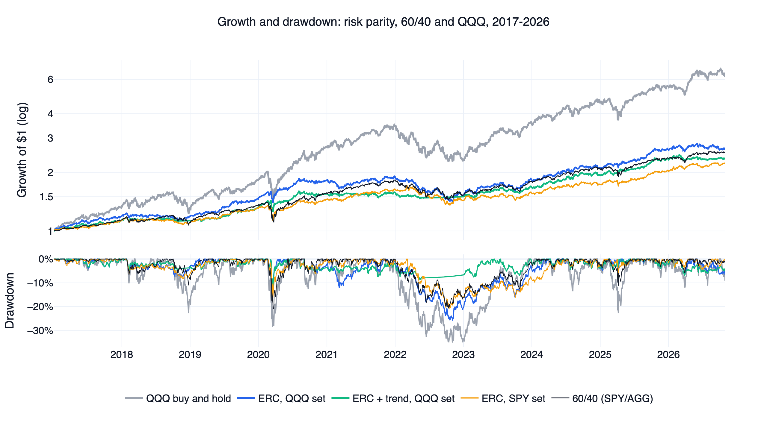
One dollar in QQQ became 2.61, ERC + trend 2.21 and 60/40 $2.52. All six designs drew down less than QQQ's -35.1%.
Result 4: bonds stopped hedging in the second half
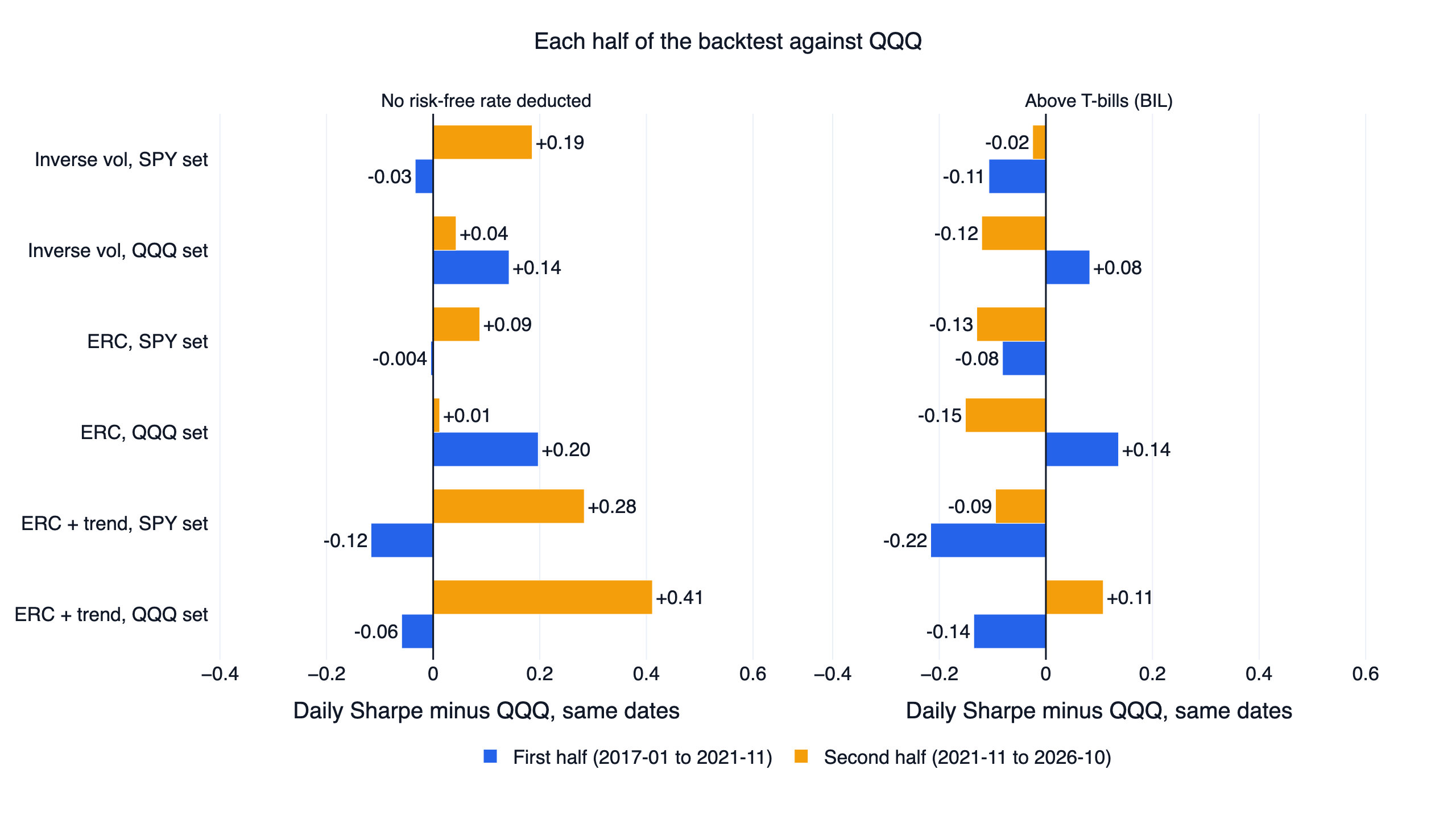
ERC on the QQQ set won the first half clearly, 1.45 against 1.25 and 1.34 against 1.21 above T-bills. In the second half it scraped 0.63 against 0.62 and lost 0.31 against 0.46 above T-bills. Five of the six designs lost the second half above T-bills; only ERC + trend on the QQQ set won it, 0.57 against 0.46.
Part of the reason is the correlation risk parity relies on. Daily, TLT moved against SPY with a correlation of -0.38 in the first half and +0.10 in the second. TLT returned 6.8% a year before the split and -8.3% a year after it. Campbell, Sunderam & Viceira (2009) explain why that sign can flip: when inflation is the main risk, rising rates hit stocks and bonds together. In 2022 QQQ lost 32.6% and TLT 31.2%, gold was flat at -0.8%, and ERC on the QQQ set lost 20.2%. ERC on the SPY set lost 12.2%: SPY fell less than QQQ, at -18.2%, and DBC gained 19.3%, the one asset here that hedged that year.
RPAR and UPAR: the listed risk parity ETFs
RPAR and UPAR are the two US-listed funds with risk parity in their names. RPAR tracks the Advanced Research Risk Parity Index across equities, commodities, Treasuries and TIPS, and its top holdings include Treasury futures, with a 0.52% net expense ratio. UPAR runs the same strategy with more leverage for a higher target return and risk, at 0.68%.
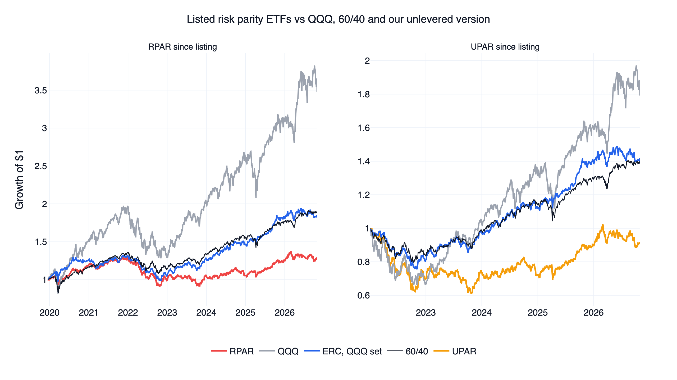
| Since RPAR's first day, 2019-12-13 | CAGR | Daily Sharpe | Above T-bills | Max drawdown |
|---|---|---|---|---|
| RPAR | 3.6% | 0.34 | 0.13 | -30.1% |
| 60/40 | 9.6% | 0.80 | 0.58 | -20.9% |
| ERC, QQQ set | 9.1% | 0.80 | 0.57 | -25.9% |
| QQQ | 19.9% | 0.86 | 0.75 | -35.1% |
| Since UPAR's first day, 2022-01-04 | CAGR | Daily Sharpe | Above T-bills | Max drawdown |
|---|---|---|---|---|
| UPAR | -2.1% | -0.03 | -0.24 | -39.0% |
| 60/40 | 7.0% | 0.66 | 0.32 | -20.5% |
| ERC, QQQ set | 7.1% | 0.65 | 0.32 | -24.6% |
| QQQ | 12.9% | 0.64 | 0.47 | -34.0% |
Listing dates decide a lot here. UPAR began just as the 2022 bond sell-off started and lost 30.3% that year; RPAR lost 22.8%. The two funds are real and pay their fees, while our lines are zero-cost backtests that hold QQQ and gold where the funds hold a broader mix, so this compares different things. RPAR's gap to ERC on the QQQ set also opened after 2022 rather than during it: RPAR returned 6.0% in 2023 and 0.1% in 2024, while ERC on the QQQ set returned 21.7% and 13.6%. We did not split that gap into leverage, TIPS and equity mix.
The code
This builds ERC and the trend filter on the QQQ set, then prints two Sharpe ratios for each and for QQQ: the first with no risk-free rate deducted, the second above T-bills.
Show Code
import finlab
import numpy as np
import pandas as pd
from finlab import data
from finlab.backtest import sim

finlab.login()
data.truncate_end = "2026-10-30"   # the article's last day; remove it for the latest data
data.set_market("us_fund")
close = data.get("us_fund_price:adj_close").dropna(subset=["SPY"])   # drop market holidays

ASSETS = ["QQQ", "TLT", "GLD"]
daily = close[ASSETS].pct_change(fill_method=None)
days = close.index
month_ends = pd.DatetimeIndex(pd.Series(days, index=days).groupby(days.to_period("M")).max().values)
signals = month_ends[month_ends >= "2016-12-30"]


# 1. Equal risk contribution from 63 days of daily returns (long only, no leverage)
def equal_risk_contribution(cov):
    n = len(cov)
    w = np.full(n, 1 / n)
    for _ in range(200):
        for i in range(n):
            others = cov[i] @ w - cov[i, i] * w[i]
            w[i] = (-others + (others ** 2 + 4 * cov[i, i] / n) ** 0.5) / (2 * cov[i, i])
    return w / w.sum()


rows = {d: equal_risk_contribution(daily.loc[:d].tail(63).cov().to_numpy()) for d in signals}
risk_parity = pd.DataFrame(rows, index=ASSETS).T

# 2. Trend filter: a slice whose asset is not above its 10-month average moves to T-bills
monthly = close[ASSETS].reindex(month_ends)
above_average = (monthly > monthly.rolling(10).mean()).reindex(signals)
with_trend = risk_parity.where(above_average, 0.0)
with_trend["BIL"] = 1 - with_trend.sum(axis=1)


# 3. Backtest at the next close; Sharpe with and without T-bills deducted
def backtest(weights):
    position = weights.reindex(days[days >= signals[0]], method="ffill")
    report = sim(position, resample="M", trade_at_price="close", upload=False)
    return report.creturn.loc["2017-01-03":]


def sharpes(curve):
    returns = curve.pct_change().dropna()
    above_bills = returns - close["BIL"].pct_change(fill_method=None).reindex(returns.index)
    return [f"{r.mean() / r.std() * 252 ** 0.5:.2f}" for r in (returns, above_bills)]


print("ERC", sharpes(backtest(risk_parity)))
print("ERC + trend", sharpes(backtest(with_trend)))
print("QQQ", sharpes(close["QQQ"].loc["2017-01-03":]))
With data to 2026-10-30 this prints 0.99 and 0.77 for ERC, 1.11 and 0.82 with the trend filter, and 0.93 and 0.83 for QQQ, matching research.py.
Run it with your AI agent
The quickest way to test your own version is to let an AI coding agent edit and rerun the script. Install the FinLab skill with npx skills add https://github.com/koreal6803/finlab-ai --skill finlab; it works with Claude Code, Codex and Gemini CLI, and the agent setup page covers each one. Then ask for one change at a time, for example "replace TLT with IEF in the QQQ set" or "lever ERC to 15% volatility and charge the T-bill rate", and have it rerun all the checks, including the one above T-bills. If you prefer not to install anything, the same research runs in FinLab Studio at studio.finlab.finance through the AI-assisted setup.
Backtest method and limits
| Item | How this study handles it |
|---|---|
| Window | First signal 2016-12-30, the first month end with 12 month-end closes behind it; first fill at the 2017-01-03 close; last day 2026-10-30. finlab's fund price table starts in January 2016, so the study cannot reach 2008 or the 1970s |
| Data | finlab us_fund_price:adj_close, closes adjusted for reinvested distributions, with the blank rows on US market holidays dropped |
| Universe | Fixed by hand before the test: SPY, TLT, GLD, DBC and QQQ, TLT, GLD, plus BIL as cash. There is no stock selection, liquidity filter or delisting risk; choosing liquid ETFs that still exist is itself a form of hindsight |
| Weights | Long only, no leverage, adding to 100%. Volatility and covariance come from daily returns up to the signal day. The leverage table is a separate calculation on the finished curves |
| Execution | Signals use the month-end close and trade at the next day's close; nothing after the signal is used (look-ahead bias). Between rebalances the weights drift |
| Costs | finlab's US fund default: no commission, no tax, no bid-ask spread. At 0.1% per side, CAGR falls from 10.3% to 10.2% for ERC on the QQQ set and from 9.0% to 8.5% with the trend filter. Slippage is not modelled beyond that test |
| Turnover | One-way turnover of the target weights, ignoring drift: 46% to 64% a year without the filter, 225% to 228% with it |
| Capacity | Not estimated. SPY, QQQ, TLT and GLD are among the most traded ETFs |
| Dividend withholding | Adjusted prices assume every distribution is reinvested in full, with no tax. Non-US investors usually pay withholding on stock ETF distributions |
| Benchmark | QQQ buy and hold with dividends reinvested, no costs, on the same dates. RPAR and UPAR run from their first day in our data, and our curves are cut to those dates |
| Sample | Everything is in-sample. The halves are a stability check. There is no out-of-sample test. 2022 is one regime change, and we did not measure how much of the result it explains |
What this result does and does not say
Under this setup, from 2017 to 2026, unlevered risk parity on these ETFs did not beat holding QQQ once T-bills were deducted. It delivered what it promises on risk: volatility of 6.8% to 10.5% against QQQ's 22.8% and drawdowns of -9.0% to -25.9% against -35.1%.
Against 60/40, its natural rival, the result is closer. Above T-bills, four of the six designs beat 60/40's 0.69, and the two ERC designs on the SPY set fell just short at 0.68 and 0.67. The QQQ set helped, and choosing QQQ over SPY is a choice made with knowledge of this decade.
This window is an unfavourable one for the idea: a long run for large US growth stocks, then the fastest rate-hiking cycle in four decades, and a data history too short to include 2008. Asness, Frazzini & Pedersen use data back to 1926. We built no version with futures, inflation-linked bonds or a broader set of assets; RPAR and UPAR are the only evidence here on that kind of portfolio.
It does give a usable rule. Any portfolio that is mostly bonds and cash needs its Sharpe checked above T-bills, and any risk parity pitch should be read at the leverage it needs and the cost of that leverage.
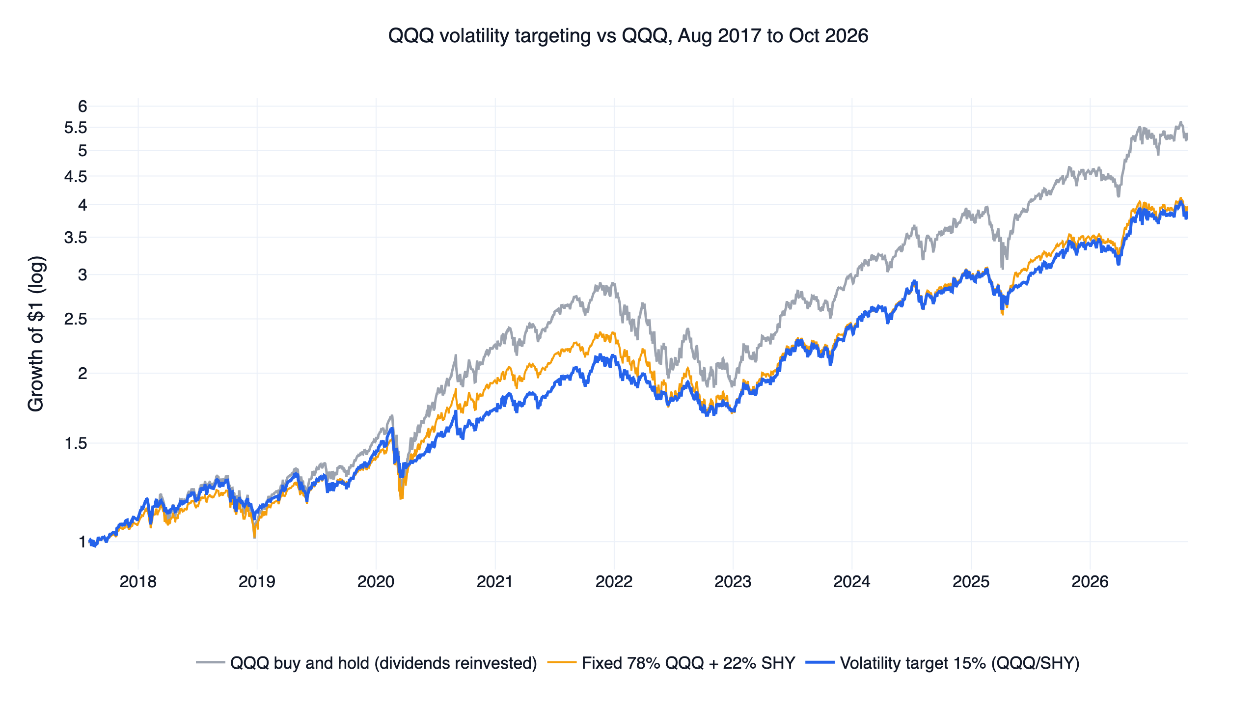
Other ways to hold US assets are covered in the QQQ volatility targeting strategy, which moves between QQQ and short-term Treasuries (SHY) and has a live strategy page, the covered call, Magnificent 7 and dividend backtest, the long-short and trend-following backtest and the ETF rotation strategy. The US quant trading strategies overview lists the rest, and the quant trading guide covers the method behind these checks.
FAQ
What is a risk parity portfolio?
A portfolio that sets each asset's weight from its risk, so that stocks, bonds, gold and commodities contribute similar amounts of volatility. Low-volatility assets get more capital. In our ERC portfolio on QQQ, TLT and GLD, TLT averaged 38% of the money and exactly a third of the risk.
Does risk parity still work?
It reduced risk, and it did not beat QQQ from 2017 to 2026 once T-bills were deducted: 0 of 54 settings did. With no risk-free rate deducted, 51 of 54 did. Five of the six designs lost the second half above T-bills, after the 2022 bond sell-off ended the negative stock-bond correlation. Four of the six had already trailed QQQ above T-bills in the first half.
What is the difference between inverse volatility and equal risk contribution?
Inverse volatility uses each asset's volatility alone. Equal risk contribution also uses correlations, so each asset's share of portfolio risk comes out equal. In our test the two were close: daily Sharpe 0.99 for both on the QQQ set, and 0.99 against 0.94 on the SPY set. Equal weights matched or beat both.
How have RPAR and UPAR performed?
From its first day in our data, 2019-12-13, to 2026-10-30, RPAR returned 3.6% a year with a daily Sharpe of 0.34 and a -30.1% maximum drawdown. UPAR returned -2.1% a year from 2022-01-04 with a -39.0% drawdown. Over the same dates 60/40 returned 9.6% and 7.0% and QQQ 19.9% and 12.9%. Both funds lost heavily in 2022, RPAR 22.8% and UPAR 30.3%.
Is risk parity the same as the All Weather portfolio?
Bridgewater's All Weather is built on similar thinking, and the retail version is a fixed mix of 30% stocks, 55% Treasuries and 7.5% each in gold and commodities. That mix scored 0.75 here. ERC, which recomputes weights monthly from recent risk on similar assets, scored 0.94.
Why deduct T-bills from the Sharpe ratio?
Because T-bills pay a return with almost no volatility, and that return adds more to the Sharpe of a calm portfolio than a volatile one. It added 0.22 to ERC on the QQQ set and 0.10 to QQQ. Leverage is also financed near the T-bill rate, so the Sharpe above T-bills shows what a levered risk parity portfolio can keep.
Does a trend filter help risk parity?
On QQQ, TLT and GLD it raised daily Sharpe from 0.99 to 1.11 and cut the worst drawdown from -25.9% to -13.0%, in exchange for about 1.3 points of annual return and more than four times the turnover. On SPY, TLT, GLD and DBC the same filter did better on equal weights than on ERC. Neither version passed.
Can I rerun this?
Yes. Install FinLab through the AI-assisted setup, download research.py below and run it; it takes under a minute with the data cached.
Reproduce it yourself
- research.py: all six designs, 54 neighbouring settings, both halves, cost runs, the T-bill measure and every control.
- data.csv: daily equity of the six designs at their original settings, the controls, RPAR, UPAR, QQQ and the single ETFs.
- metrics.json: every statistic quoted here, including each setting, both halves, month-end weights and yearly returns.
Last updated: 2026-11 | Backtest window: 2017-01 to 2026-10 | Benchmark: QQQ total return | Author: FinLab Quant Research (reviewed by a quantitative researcher)
Past performance does not represent future results, and every result here is an in-sample backtest. The ETFs named are used to describe research results, not as recommendations. This content is for education only and does not constitute investment advice.
FinLab AI
Want to build your own strategy?
Describe your stock-picking ideas in natural language. AI automatically validates, backtests, and gives you answers
Start Free