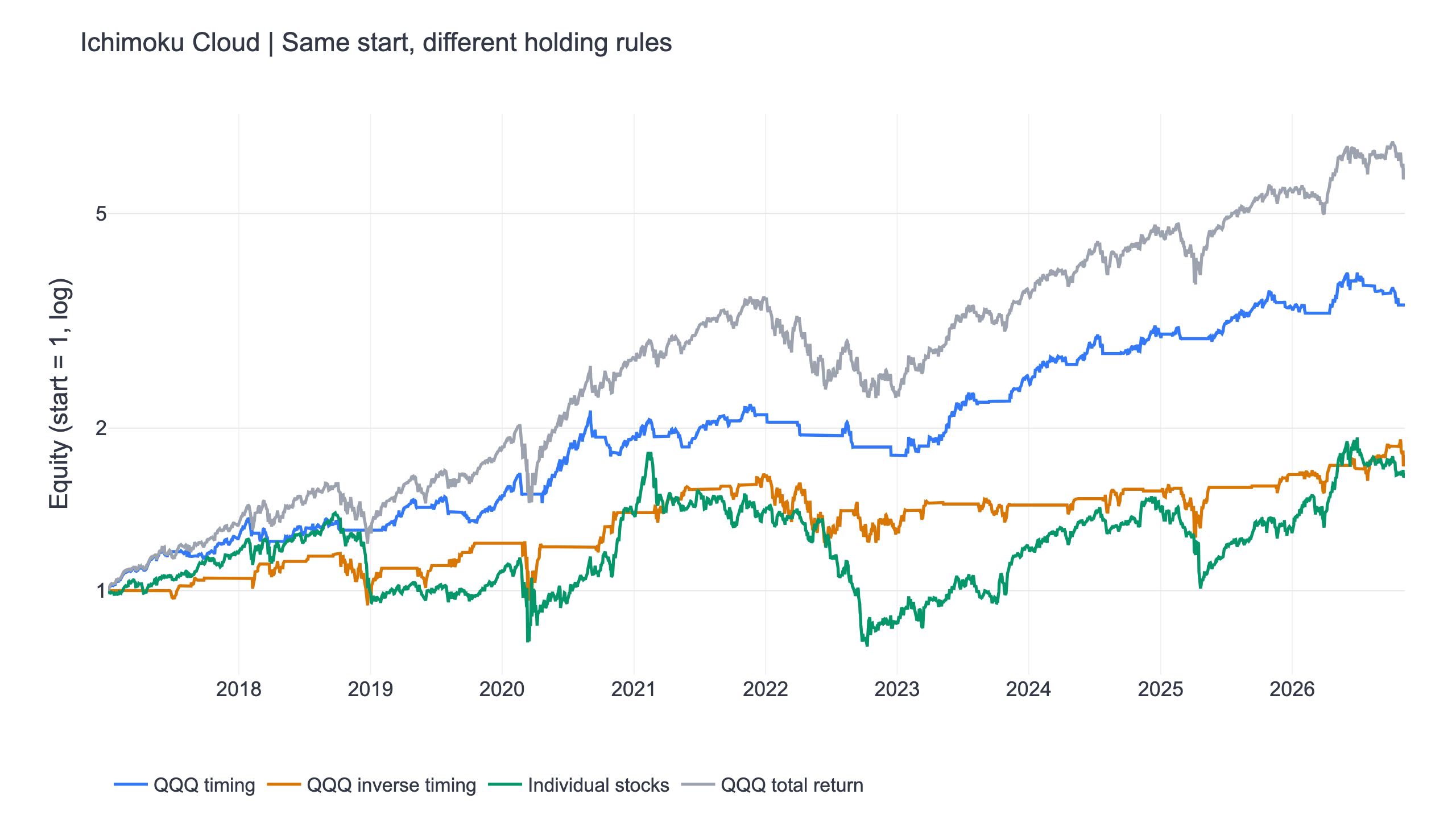
None of the three Ichimoku Cloud designs passes the full validation. QQQ timing wins all nine zero-commission parameter comparisons and both halves, but fails when 0.1% per-side costs and BIL are included together: excess-return daily Sharpe is 0.745, below QQQ's 0.814. This is a failed trading hypothesis, not a validated strategy to deploy.
The stock version returned 5.1% a year and won 0 of nine parameter comparisons. Applying the indicator to individual companies did not reproduce a robust advantage over QQQ. The figure compares all three central rules with the benchmark from the same starting value; click it for the full-size chart.
These trading rules are research results. To rerun the experiment, set up FinLab and download the research program (.py). Other files are in the research downloads.
Ichimoku Cloud strategy: what the five lines mean
Ichimoku Cloud describes price relative to several high-low midpoints. A midpoint uses the highest high and lowest low over a window. It gives the same weight to the two extremes; it does not average every closing price. That distinction matters after a short-lived spike, because an extreme can keep affecting the line until it leaves the window.
The conversion line measures the shorter window. The base line measures the intermediate window. Leading span A is the midpoint of those two lines; leading span B is the midpoint over the longer window. The two spans enclose the cloud. The familiar chart draws them forward, while the lagging span draws today's close back in time. Those drawing conventions describe where a value appears on a chart. They do not change when the value became known.
| Component | Calculation used here | Trading role |
|---|---|---|
| Conversion line | Nine-session high-low midpoint | Must be above the base |
| Base line | Twenty-six-session high-low midpoint | Intermediate trend comparison |
| Leading span A | Average of conversion and base, shifted forward 26 sessions | First cloud boundary |
| Leading span B | Fifty-two-session high-low midpoint, shifted forward 26 sessions | Second cloud boundary |
| Lagging span | Today's close plotted in the past | Excluded from this rule |
A close must be above both cloud boundaries, and the conversion line must exceed the base line. Equality does not qualify. The account holds QQQ while all three conditions hold and cash when any condition fails. This is a state rule, so there is no requirement to wait for a fresh crossover before reentering. It also does not require a green cloud, a particular cloud thickness or a separate confirmation from the lagging span.
Forward plotting and future leakage
At session t, the cloud displayed at t was calculated 26 sessions earlier. The code therefore uses a positive shift(26). Shifting the data backward would import later information into an earlier decision. Using the undisplaced span would be a different strategy, even though every input would still be historical. The experiment fixes the displaced definition before looking at returns.
The longer midpoint and its displacement also require a warm-up period. Prices from 2016 supply that history for the US experiment; performance starts in 2017. Nontrading rows are removed using QQQ's available-price calendar before rolling windows are calculated. Keeping empty holiday rows would make a 52-session window fail repeatedly and could quietly turn an apparent decade-long experiment into a much shorter one.
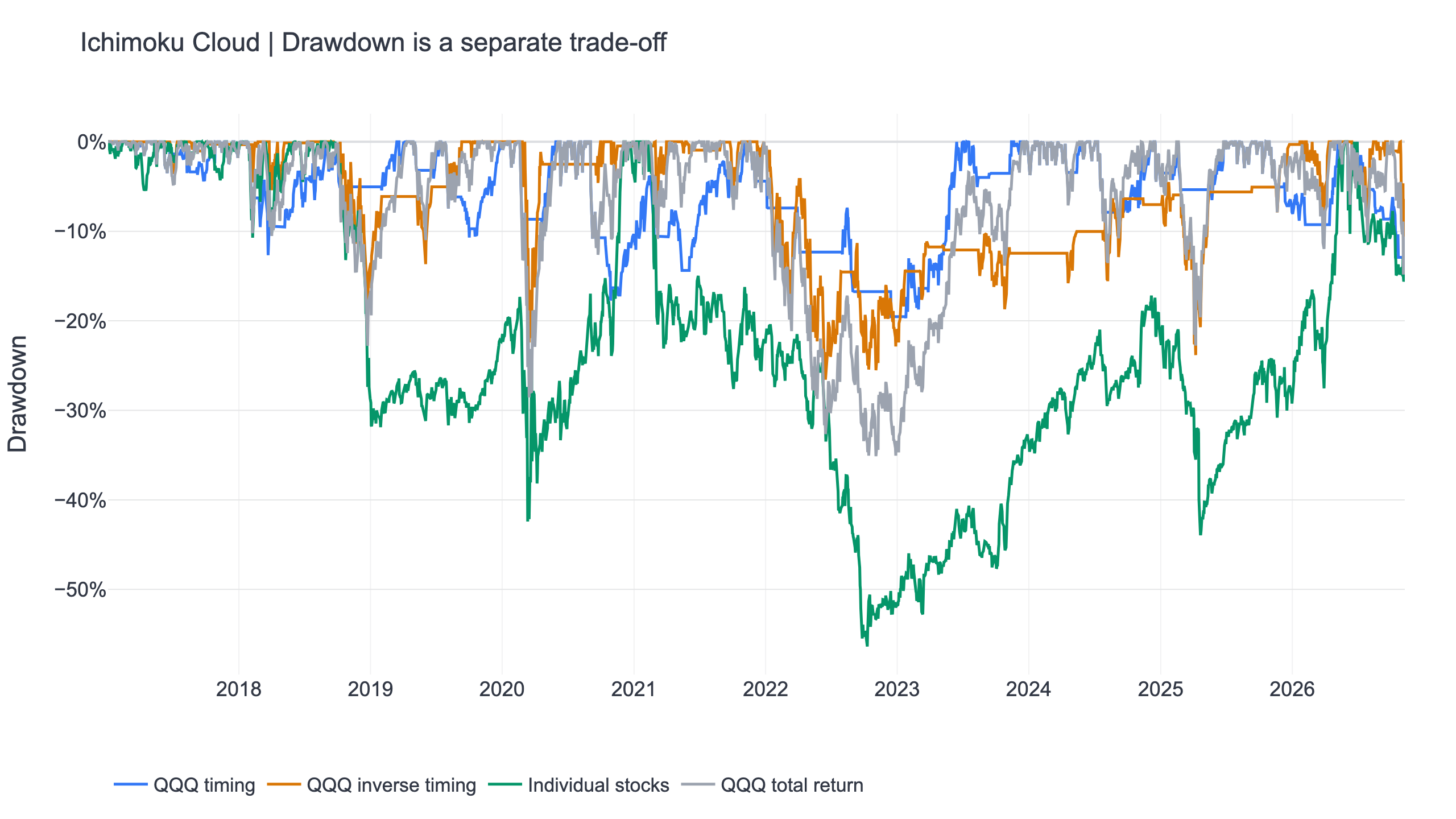
A cloud can sit below a price that is already falling. It is built from earlier extremes, so the rule responds after price changes, with an additional delay before execution. The shallower drawdown in this QQQ sample does not turn the cloud into an advance warning system. The individual-stock comparison is useful precisely because it shows whether the same visual construction transfers to another way of holding securities.
Reading an Ichimoku chart without changing this experiment
A thin cloud, a bullish cloud twist and a bounce from the base line are common chart interpretations. None enters this test. Adding one after seeing a bad year would change the hypothesis and require a separately registered experiment. The nine settings ask a smaller question: does a nearby family of the same cloud rule retain a risk-adjusted advantage after realistic comparisons?
A favorable result also has an opportunity cost. When the rule sits in cash during a rising market, it misses part of the advance. Comparing only the worst drawdown would hide that cost. The annual return column, the inverse-timing portfolio and the exposure control show what was given up. For investors whose objective is maximum equity participation, a lower-return defensive rule may still be the wrong fit.
The Japanese Technical Analysts Association attributes Ichimoku to Goichi Hosoda, who used the pen name Ichimoku Sanjin. The present experiment tests a narrow, mechanical subset of that charting approach. Original source.
Results: all three holding designs
| Central design | Annualized return (CAGR) | Daily Sharpe | Max drawdown | First / second half Sharpe | Settings beating QQQ | Time invested |
|---|---|---|---|---|---|---|
| QQQ timing | 13.2% | 1.02 | -19.7% | 1.2178 / 0.8172 | 9 / 9 | 61.5% |
| QQQ inverse timing | 6.1% | 0.41 | -26.6% | 0.6039 / 0.2283 | 0 / 9 | 38.4% |
| Individual stocks | 5.1% | 0.33 | -56.4% | 0.4276 / 0.2182 | 0 / 9 | 99.8% |
| QQQ total return | 20.1% | 0.92 | -35.1% | 1.2172 / 0.6316 | — | 100% |
Daily Sharpe here means average daily return divided by its standard deviation, multiplied by the square root of 252, without subtracting a risk-free rate. CAGR uses elapsed calendar years. Maximum drawdown is the deepest fall from a previous equity peak. These are different questions, so a higher Sharpe does not imply a higher annual return. Sharpe (1994) defines the ratio using differential returns; the zero-rate convention here is explicit.
The embedded FinLab report is the central QQQ timing rule, not the best-performing grid cell. The second downloadable report is the central stock portfolio. The headline table keeps the full common window, including cash before the first trade; a report can begin at its first executed trade. Its built-in Sharpe also has its own risk-free-rate convention, while this study's comparisons consistently use zero.
Neighboring parameters and the two halves
Conversion length 7, 9 or 11 sessions; base length 22, 26 or 30. The long span is twice the base length and displacement equals the base length. The center is 9/26/52 with a 26-session displacement. Every combination was registered before reviewing results. At least seven of the nine settings must beat QQQ's same-window daily Sharpe. The central setting must also beat it in each half of the trading-day calendar. These are robustness screens on historical data, not untouched out-of-sample forecasts.
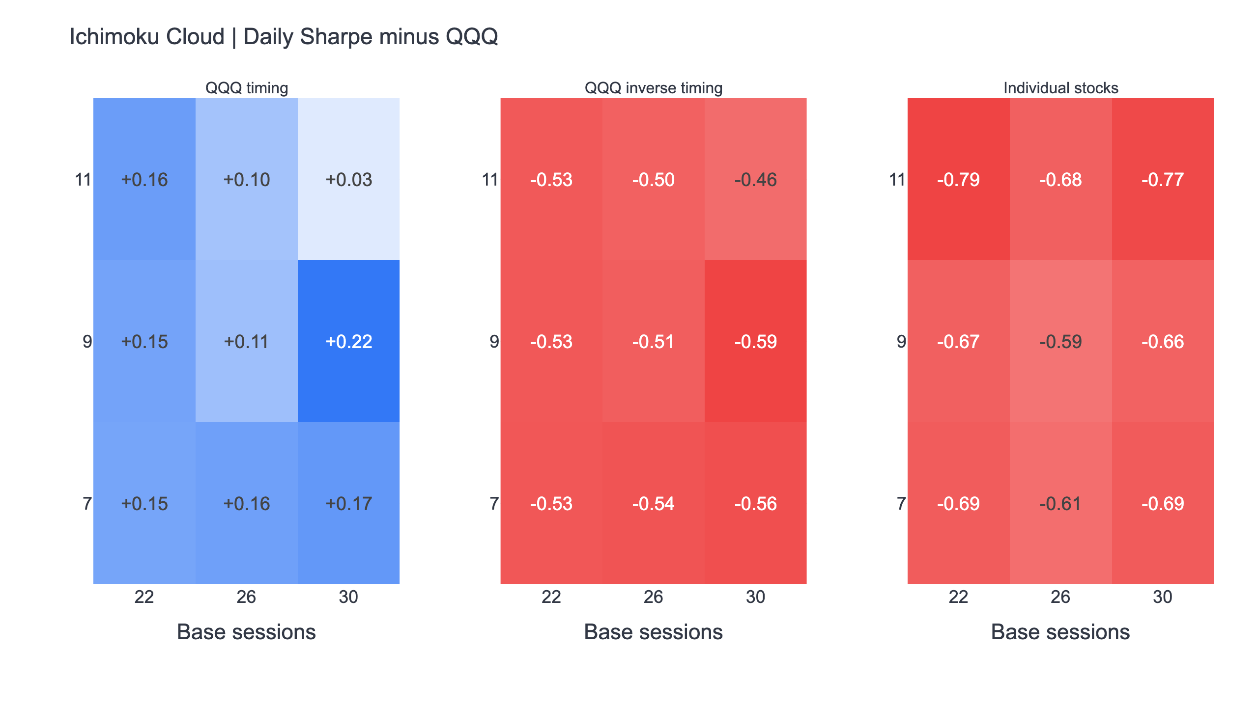
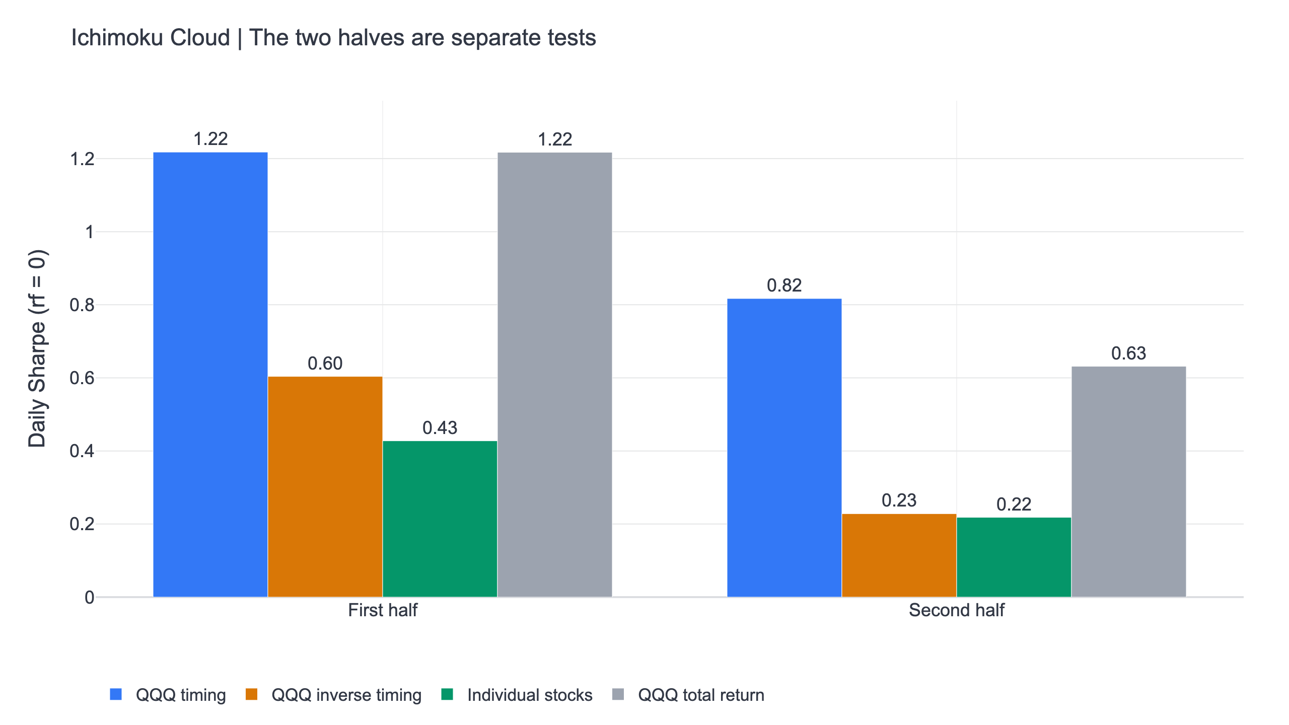
Blue positive cells beat the benchmark; negative cells do not. The three panels belong to timing, inverse timing and stock holding. The split-period chart compares those same central allocations with QQQ rather than changing parameters between periods. A full-window lead cannot compensate for a failed half or an unstable neighborhood.
Costs, cash and the best year
The US market default in sim() is zero commission and zero transaction tax. Each central rule is also rerun with 0.1% per side, a separate allowance for trading friction. No additional market-impact model, tax-on-capital-gains calculation or capacity estimate is supplied.
The equity curves, parameter grid, split-period chart and embedded report use zero commission. In the table, the first two numeric columns include 0.1% per-side costs; the BIL column is the separate zero-commission comparison. The joint cost-and-BIL check for the Ichimoku candidate is detailed below.
| Central rule | CAGR at 0.1% per side | Daily Sharpe at 0.1% | Zero-fee Sharpe after BIL | Best calendar year removed | Sharpe without that year / QQQ |
|---|---|---|---|---|---|
| QQQ timing | 11.8% | 0.93 | 0.84 | 2023 | 0.84 / 0.78 |
| QQQ inverse timing | 4.8% | 0.34 | 0.28 | 2019 | 0.32 / 0.83 |
| Individual stocks | -0.9% | 0.08 | 0.23 | 2023 | 0.20 / 0.78 |
Subtracting BIL's daily total return gives QQQ an excess-return Sharpe of 0.81. Idle cash earns zero in the strategy; the experiment does not quietly pay Treasury returns to cash holdings. The fixed-exposure control holds the same average fraction of QQQ every day and keeps the remainder at zero-return cash. Its Sharpe for the timing allocation is 0.92, compared with 1.02 for the rule. The control excludes rebalancing costs.
Removing the central rule's best calendar year is an additional historical stress test. That year is selected from the rule's own annual returns, and the same dates are removed from the benchmark. The remaining daily returns are compounded without inserting a return across the removed interval. Passing this check cannot repair an earlier failure.
Why the apparently passing QQQ rule still fails
The zero-commission timing Sharpe is 1.0229 versus QQQ's 0.9172, and all nine nearby settings win. Its first-half lead is only 1.2178 versus 1.2172, about 0.0005. At 0.1% per side, timing falls to 0.9267, narrowly above QQQ before deducting the cash benchmark. That apparent lead is insufficient: subtracting BIL from the same cost-stressed returns produces 0.7455 versus QQQ's 0.8143.
The strategy spends about 38% of sessions in zero-return cash. A full-account cash benchmark remains relevant during those sessions. Showing the cost test and the BIL test separately would miss their combined effect. The joint check fails, so this study does not create a strategy page or a validated-strategy Studio shortcut. The small first-half margin also should not be read as statistical significance. Removing the best year does not repair the cost-and-cash failure.
Universe, execution and limits of the evidence
Signals are formed after the close and executed at the following trading session’s market close in every grid and central rule.
The data end on 2026-11-09 and this run was completed on 2026-11-11, using finlab 2.3.8. US adjusted OHLC comes from us_price for stocks and us_fund_price for QQQ. QQQ's adjusted close is the total-return benchmark, computed directly from prices without transaction costs. Every comparison uses its available trading calendar.
The stock universe uses FinLab's common-stock classification, adjusted price above 5 million, and the 100 largest such amounts each day. The amount requires at least 20 observations. A stock is excluded after a 50% absolute daily move, using a rolling 252-session record shifted by one session. This screens earlier extreme moves; it cannot prevent the first extreme event. The common-stock classification is a present security-type filter, so historical classification changes remain a limitation.
Eligible stocks with positive indicator states receive equal target weights, recalculated daily. The market, liquidity ranking and indicator use information available at that close. No present-day S&P 500 membership list, analyst snapshot, financial-statement factor or investor's private strategy is used. Available delisted price columns are retained when they pass classification, but completeness of delisting returns is not separately audited. Financial and other sectors are not individually excluded, and there is no market-cap forecast or sector-neutral constraint.
Each stock receives 1 divided by the number of current holdings; no additional per-stock cap is imposed, so a single remaining stock can receive 100%. The fund rules allocate either 100% to QQQ or 100% to cash. Target-weight turnover for each central allocation is:
| Central allocation | Recorded trades | Average monthly target turnover | Highest month |
|---|---|---|---|
| QQQ timing | 61 | 50.8% | 300.0% |
| QQQ inverse timing | 61 | 50.8% | 300.0% |
| Individual stocks | 4696 | 242.7% | 545.2% |
The central stock version averages 28.4 positions. Target-weight turnover is half the absolute daily target-weight changes, summed by month. This is not executed notional turnover: price drift and execution details can change the actual amount. A change in universe membership can require trading even without a fresh indicator reversal.
All tests are historical and in sample. Registering parameters before this run reduces within-batch cherry-picking, but the idea and market were selected with knowledge of financial history. The half-period split, grid and best-year check do not provide a statistical probability of future profit. Bailey and colleagues (2017) examine backtest overfitting; this study does not estimate their probability-of-overfitting statistic. Moskowitz, Ooi and Pedersen (2012) study futures trend following, which does not validate this indicator.
Reproduce the rule with an AI agent
Complete the FinLab setup flow with Claude Code, Codex or Gemini CLI. The agent guide explains how the skill gives your agent access to FinLab's data and backtests. The direct skill install command is:
Show Code
npx skills add koreal6803/finlab-ai --skill finlab -g -yThe browser version, FinLab Studio, also supports AI research. Ask the agent to reproduce the fixed experiment before proposing changes: “Use the downloaded Ichimoku Cloud research program, keep its registered dates and nine settings, and compare the three holding rules with QQQ including the cost test.” The point is to retain the definitions in the results table. A newly generated trading rule, even if it uses the same indicator name, does not reproduce this experiment.
Download the research program as research.py in the working directory. This excerpt runs the central individual-stock rule; the program's command-line options also run the complete grid. Its dependency command includes finlab, numba and TA-Lib. Login is handled by FinLab.
Show Code
import finlab
from research import load, signal, backtest

finlab.login()
prices, eligible = load("us")
state = signal(prices, "ichimoku", 9, 26)
position = (state & eligible).loc["2017-01-03":"2026-11-09"]
report = backtest(position)
report.to_html("ichimoku_stocks_report.html")
Questions about this Ichimoku Cloud test
What is the best setting? The middle values were fixed in advance. The heatmap supplies every neighboring outcome; no winning cell is substituted for the original rule.
Does a smaller drawdown prove the signal works? Cash can reduce both drawdown and return. The fixed-exposure and BIL comparisons ask whether the timing adds more than that reduction in participation.
Does the inverse rule mean short selling? No. It holds QQQ in the original rule's cash sessions and holds cash otherwise. Borrow fees and short-position losses are outside this experiment.
Can these results be transferred to an individual stock? The separate stock portfolio already tests a liquid universe, and its failure does not support selecting a few attractive charts afterward. Company-specific concentration adds another risk.
Does the report's Sharpe equal the table's? Not necessarily. This table consistently uses daily returns with a zero risk-free rate and a common full window. Report conventions and a first-trade start can differ.
Can I change the timeframe to intraday? That requires another dataset and new execution assumptions. Daily highs and lows cannot identify the order of intraday fills or guarantee fills at indicator boundaries.
For broader context, the US strategy studies distinguish validated rules from negative experiments. Backtesting methods explain execution and bias; the quant glossary defines the result metrics. The Bollinger Bands study tests a different volatility envelope, and Turtle trading tests channel breakouts. FinLab's research workflow and team information provide product and author context.
Research downloads
| File | Contents |
|---|---|
| Download research program (Python) | Give this to your AI agent after setting up FinLab |
| Download daily balances (CSV) | Daily balances for the rules and benchmark; opens in a spreadsheet |
| Download complete test results (JSON) | Full test results for AI or coding tools |
| Open timing report (web) | Interactive webpage; no setup or installation needed |
| Open stock report (web) | Interactive webpage; no setup or installation needed |
Past performance does not guarantee future results. This material is for research and education and is not investment advice. It does not recommend any individual stock, guarantee a stop price or promise that a historical advantage will persist.
Last updated: 2026-11 | Backtest window: 2017-01-03 to 2026-11-09 | Author: FinLab Quant Research. The team maintains reproducible Taiwan and US market studies using FinLab data.
FinLab AI
Want to build your own strategy?
Describe your stock-picking ideas in natural language. AI automatically validates, backtests, and gives you answers
Start Free