Run this strategy
Copy the prompt to reproduce the evidence above with the article’s data, assumptions, and risk checks.
Tell your AI:
Set up FinLab and rerun the S&P 500 Bollinger Bands backtest. Please read: https://finlab.finance/en/setup?relatedUrl=/en/blog/bollinger-bands-strategy-backtest
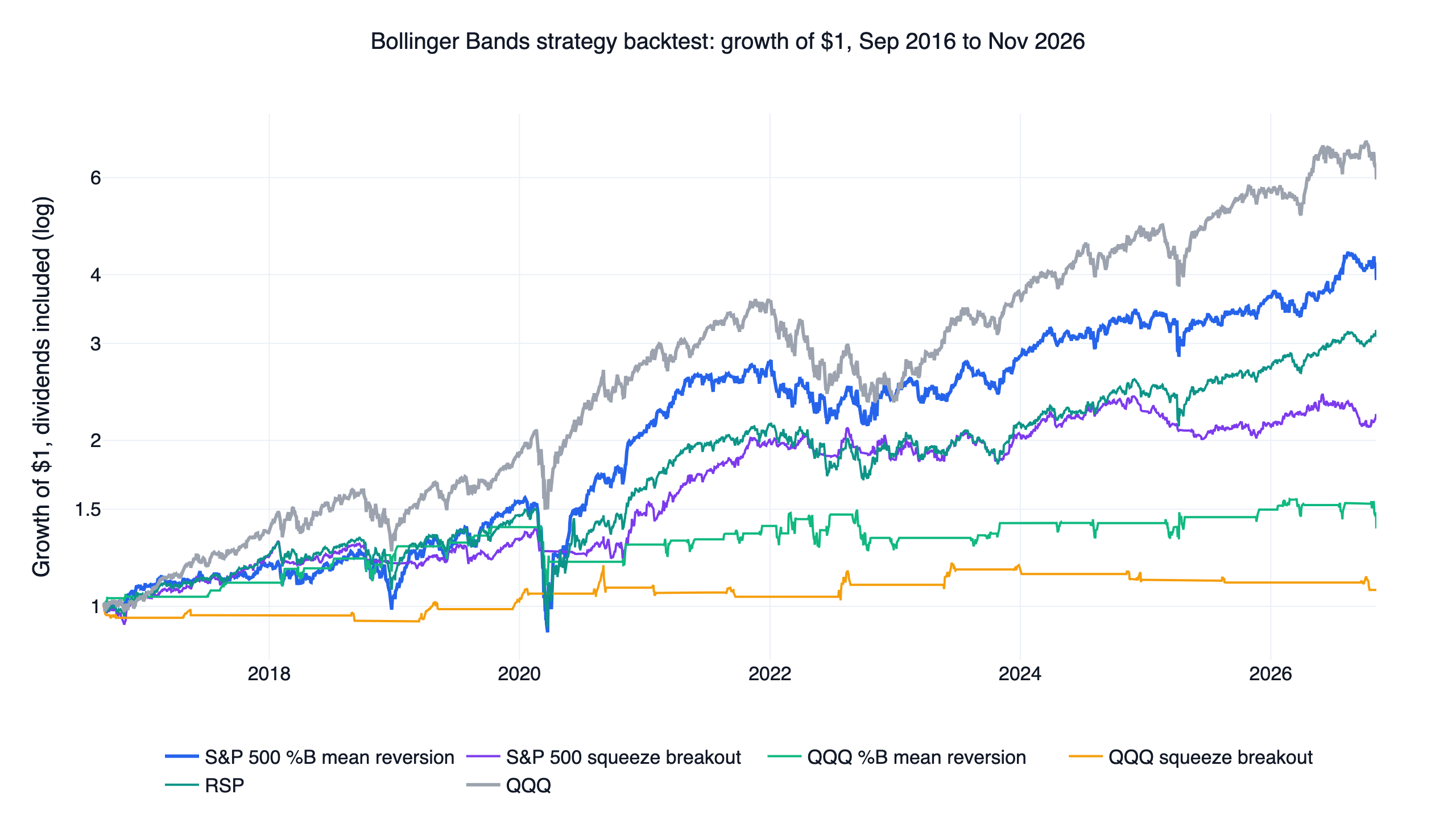
We tested four Bollinger Bands strategies on US stocks from September 2016 to November 2026, and none of them beat buying QQQ. The best was the classic mean reversion trade on individual S&P 500 stocks: buy when a stock closes below its lower band, sell when it gets back to the middle band. It returned 14.3% a year with a daily Sharpe ratio of 0.75, ahead of RSP, the equal-weight S&P 500 fund (11.7% and 0.70), and behind QQQ with dividends (19.2% and 0.89). It also turned the portfolio over 33 times a year, and at 0.1% per side its return fell to 6.9%. The Bollinger Band squeeze and both rules on QQQ itself did worse, and none of 36 settings beat QQQ.
Bollinger Bands are usually read one chart at a time. Here the rules run on every stock in the S&P 500 on each day it was a member, and on QQQ, with the bands, entries, exits and pass conditions fixed before any result was seen.
Bollinger Bands strategy results at a glance
| Design | Daily Sharpe | CAGR | Max drawdown | Beat QQQ | Beat RSP | First / second half Sharpe | Sharpe at 0.1% per side |
|---|---|---|---|---|---|---|---|
| S&P 500 %B mean reversion | 0.75 | 14.3% | -43.0% | 0 / 9 | 5 / 9 | 0.95 / 0.52 | 0.43 |
| S&P 500 squeeze breakout | 0.70 | 8.0% | -16.8% | 0 / 9 | 3 / 9 | 1.11 / 0.32 | 0.34 |
| QQQ %B mean reversion | 0.29 | 3.3% | -22.4% | 0 / 9 | 0 / 9 | 0.43 / 0.13 | 0.24 |
| QQQ squeeze breakout | 0.15 | 0.7% | -13.7% | 0 / 9 | 0 / 9 | 0.16 / 0.13 | 0.09 |
| RSP, total return | 0.70 | 11.7% | -39.0% | reference | 0.77 / 0.62 | ||
| SPY, total return | 0.85 | 14.5% | -33.7% | reference | 0.93 / 0.76 | ||
| QQQ, total return | 0.89 | 19.2% | -35.1% | benchmark | 1.16 / 0.64 |
The stock rules and the funds run from 2016-09-01 to 2026-11-05 with dividends reinvested, and the halves split at 2021-10-01. The two QQQ rules start on their first trade, 2016-09-09 and 2016-09-06, and are compared with QQQ over their own dates (QQQ's Sharpe is 0.90 and 0.89 there).
What Bollinger Bands, %B and the squeeze measure
John Bollinger describes the bands in Bollinger on Bollinger Bands (2001): a middle band that is an N-day moving average, with an upper and a lower band k standard deviations away. The common setting is 20 days and k = 2. Two readings come from them.
- %B places the close between the bands: 0 at the lower band, 0.5 at the middle band and 1 at the upper band. A close below the lower band has a %B under 0.
- BandWidth is the distance between the upper and lower bands divided by the middle band. It shrinks when prices go quiet. A squeeze is BandWidth at its lowest in about six months, a quiet stretch that often comes before a bigger move in either direction.
Those readings give the two best-known Bollinger Bands strategies. One buys weakness at the lower band and expects the price to return to its average. The other waits for a squeeze and buys the breakout through the upper band.
The four rules we tested
- S&P 500 %B mean reversion. Buy a member when it closes below its lower band. Sell when it closes at or above the middle band (%B of 0.5 or more) or leaves the index.
- S&P 500 squeeze breakout. Buy a member when it closes above its upper band and its BandWidth was at a 126-day low on at least one of the previous 20 days. Sell when it closes below the middle band or leaves the index.
- QQQ %B mean reversion and QQQ squeeze breakout. The same two rules on QQQ alone, fully in QQQ while a trade is open and in cash otherwise.
Each rule ran on a 3 × 3 grid: N of 15, 20 or 25 days and k of 1.5, 2 or 2.5, with 20 days and 2 as the original setting. The bands use the population standard deviation, as Bollinger does. The stock rules hold every qualifying member at equal weight with at most 5% in one stock, so they keep cash when fewer than 20 stocks qualify.
How a rule had to pass
"Beat" means a higher daily Sharpe ratio than QQQ with dividends reinvested over exactly the same days. Sharpe here is the mean daily return over its standard deviation, annualised with √252, with no risk-free rate subtracted. All six conditions were written down before any result was seen.
- Neighbouring settings. At least 70% of the 9 settings had to beat QQQ.
- Both halves. The original setting had to win in each half of the window.
- Costs. It had to win at finlab's default US cost of zero and at 0.1% per side.
- No single year. It had to stay ahead after removing the calendar year of its largest lead.
- The same exposure held fixed. It had to beat its own fund held at the rule's average invested share, with the rest in cash and a monthly rebalance: QQQ for the QQQ rules, RSP for the stock rules.
- Cash. Each rule can sit in cash, so it also had to beat QQQ on returns above T-bills (BIL).
Every rule failed the first four. Both S&P 500 rules passed the fifth, the squeeze by 0.002.
S&P 500 %B mean reversion: ahead of RSP, behind QQQ
On a typical day the rule held 93 stocks, and 118.5 on average. On 2020-03-16 it held 478, nearly the whole index, because almost every member had closed below its lower band. It had fewer than 20 stocks on only 85 days, so it was 98.6% invested on average. That is also why its maximum drawdown, -43.0%, was deeper than RSP's -39.0% and QQQ's -35.1%: in a crash the rule keeps buying stocks as they fall through their bands, and it sells only when they recover to the middle band.
Over the ten years it closed 22,631 trades. 69.1% made money, with a median gain of 2.19% and a median holding period of 12 trading days. The mean gain was 0.90%, less than half the median, because the losing trades were much larger than the winning ones. The win rate alone says little about this rule.
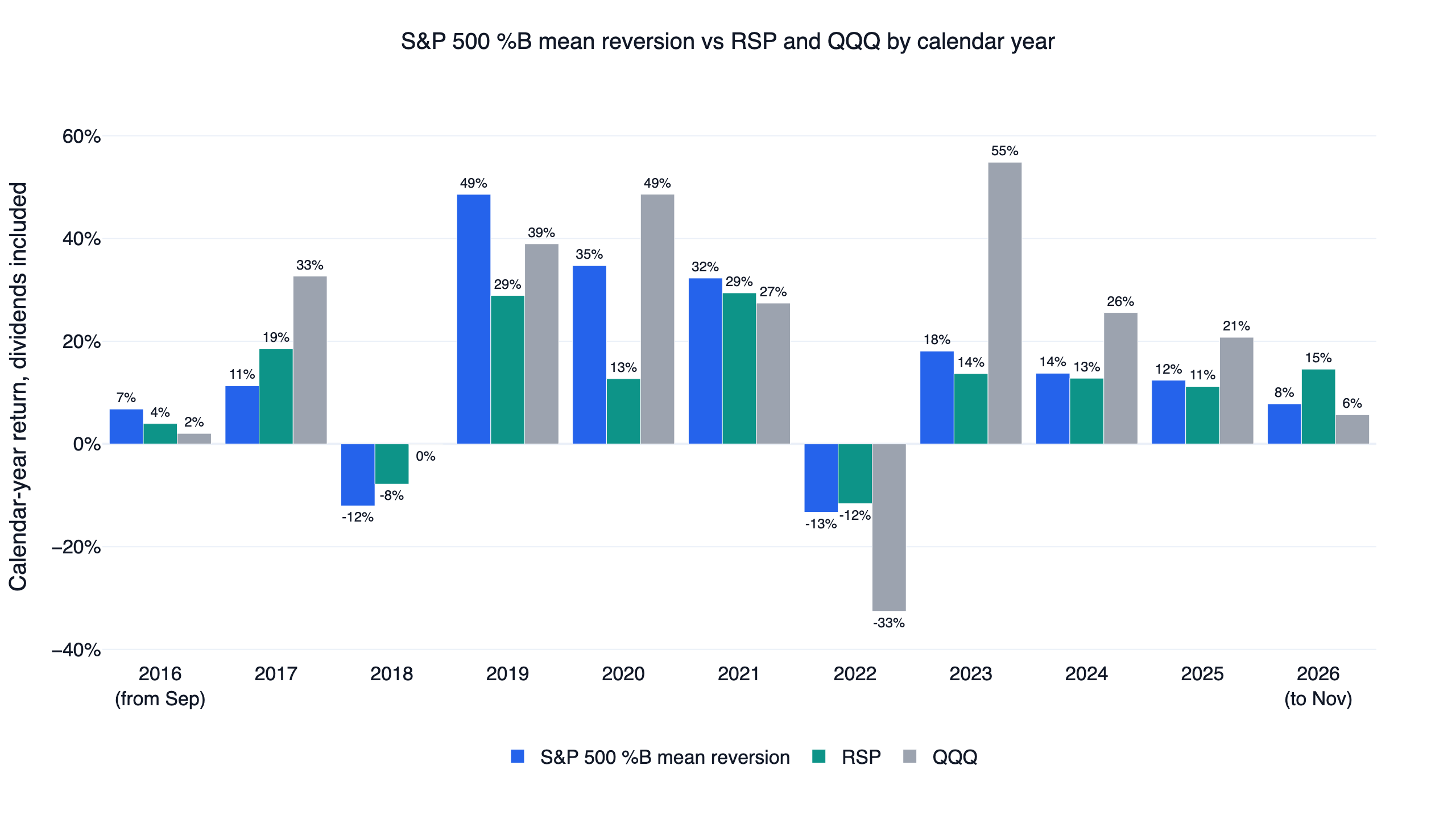
The edge over the equal-weight index was real but small. The Sharpe ratio was 0.75 against RSP's 0.70, and RSP held at the rule's 98.6% average exposure scored 0.70. Five of the nine settings beat RSP, and the 25-day bands scored lower (0.59 to 0.67). The rule's best years against RSP were 2020 (34.7% against 12.7%), 2019 (48.6% against 28.9%) and 2023 (18.1% against 13.7%). It lagged most in 2017 (11.3% against 18.5%), 2026 to date (7.8% against 14.6%) and 2018 (-12.0% against -7.8%). Its largest lead over QQQ came in 2022, when it lost 13.3% and QQQ lost 32.6%. Without 2022 its Sharpe was 0.92 against QQQ's 1.23.
The pattern fits the short-term reversal in individual stock returns. Jegadeesh (1990) found that monthly returns of US stocks tended to reverse the next month, and Lehmann (1990) found reversals at a weekly horizon. A close below the lower band is a short-term loser, and the rule collects the bounce.
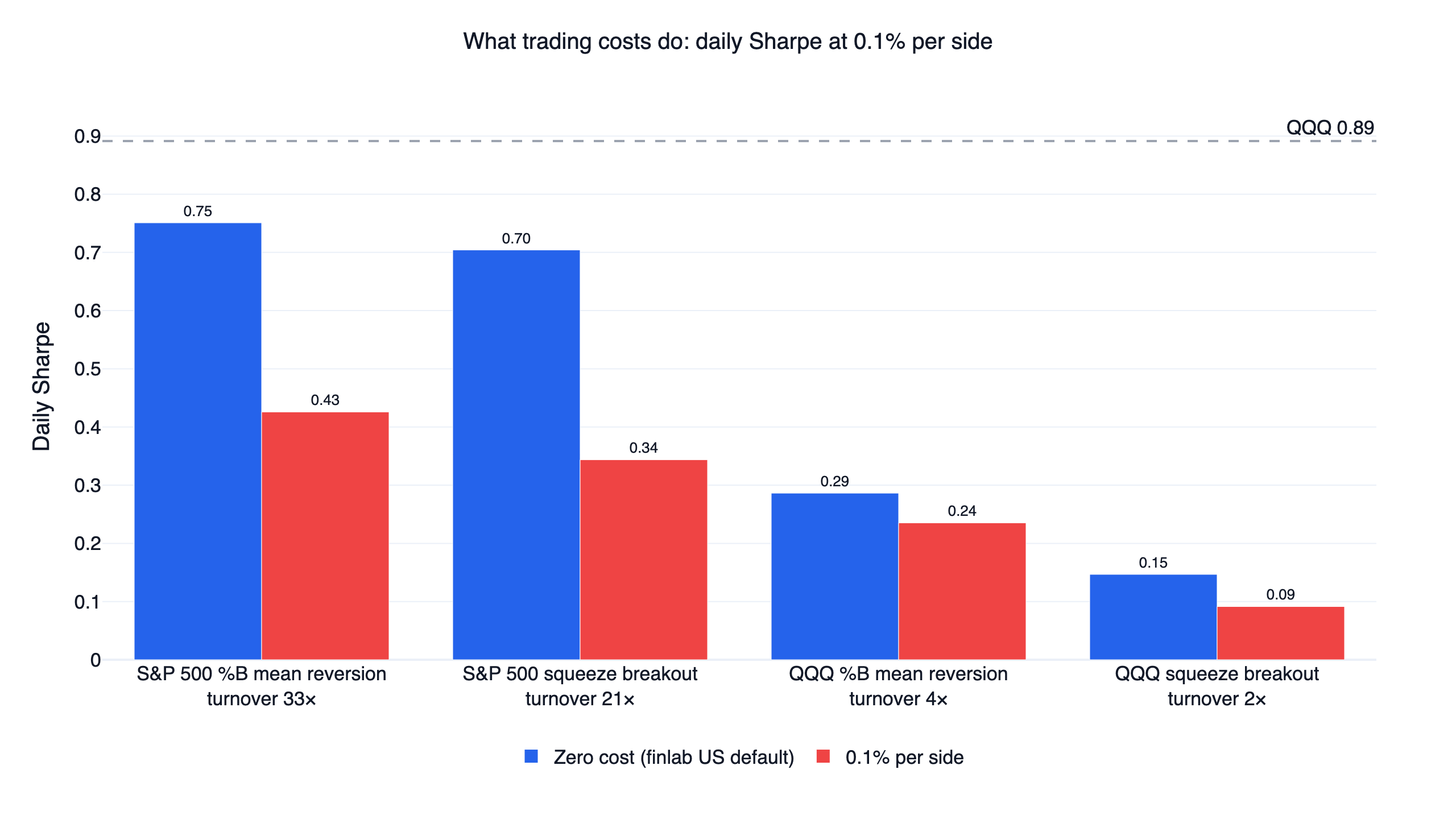
The bounce is small, so costs decide the result. Target weights turned over 33 times a year one way. At 0.1% per side that is about 6.7% of the account a year, close to the drop in return from 14.3% to 6.9%, and the Sharpe ratio fell from 0.75 to 0.43, below RSP. Turnover this high also means that real slippage matters more than the commission.
The Bollinger Band squeeze: lower risk, lower return
The squeeze rule held 34 stocks on a typical day and 39.5 on average, and it had fewer than 20 on 754 days, so it was 81.7% invested on average. It carried far less risk than the mean reversion rule, with 11.9% volatility and a maximum drawdown of -16.8% against 20.8% and -43.0%. It also returned less, 8.0% a year.
Its 6,716 closed trades show the breakout profile. Only 37.3% made money and the median trade lost 1.39%, while the mean trade gained 0.33%, so a minority of large breakouts paid for many small failures. The Sharpe ratio of 0.70 matched RSP's 0.70 and edged past RSP held at the rule's 81.7% exposure, 0.704 against 0.702. The first half came close to QQQ at 1.11 against 1.16, and the second half fell to 0.32 against 0.64. The best setting, 25 days and k = 2, scored 0.78. Turnover was 21 times a year, and at 0.1% per side the Sharpe ratio fell to 0.34.
Bollinger Bands on QQQ: rarely in the market
QQQ seldom closes below its lower band and stays there long. The mean reversion rule closed 39 trades in ten years and held QQQ on 18.2% of days. 79.5% of its trades made money, with a median gain of 1.66%, yet it returned 3.3% a year with a Sharpe ratio of 0.29. The same average exposure held every day, 18.2% of the account in QQQ and the rest in cash, scored 0.90, three times the rule's Sharpe ratio. Its maximum drawdown of -22.4% is large for an investment that was idle most of the time, because a dip bought early in a sell-off is held until the price climbs back to the middle band, with no stop.
The squeeze rule on QQQ traded 16 times, won 37.5% of them and held QQQ on 10.2% of days. It returned 0.7% a year with a Sharpe ratio of 0.15, and its nine settings ranged from -0.36 to 0.48.
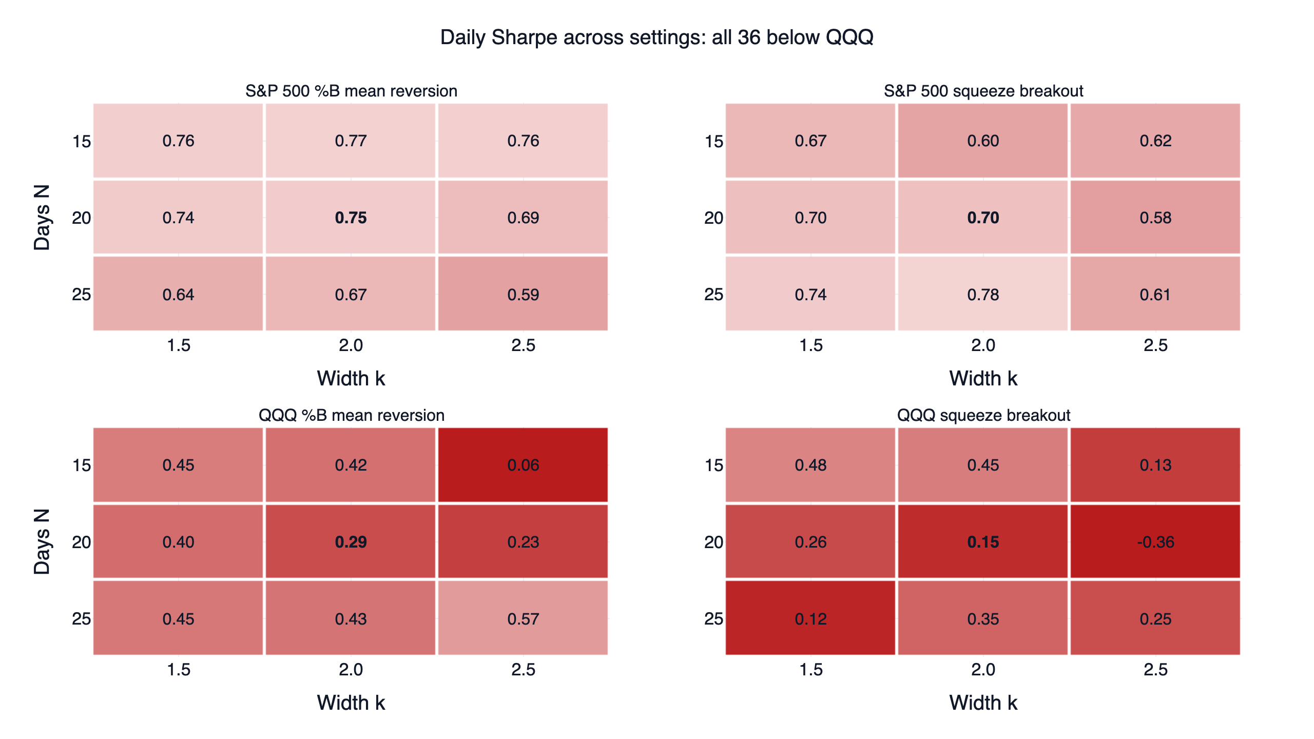
Bold marks the original settings. All 36 cells are below QQQ. The stock rules move in a narrow band (0.58 to 0.78), so 20 days and 2 standard deviations are not a sharp peak, and there is no plateau above QQQ either. The QQQ rules jump around because a few trades decide each cell.
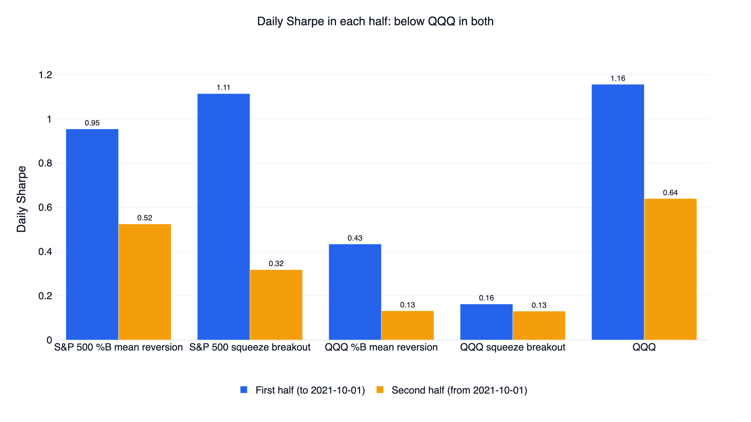
Both stock rules did better in the first half, when RSP also scored higher (0.77 against 0.62). Neither beat QQQ in either half.
How this fits other research
Technical trading rules have a mixed record. Park and Irwin (2007) reviewed 95 modern studies: 56 reported profits, 20 reported none and 19 were mixed, and they noted that many tests suffered from data snooping, rules picked after the fact, and rough estimates of risk and trading costs. A fixed rule, a fixed grid and a cost rerun are meant to address those problems, and here the Bollinger rules did not survive them.
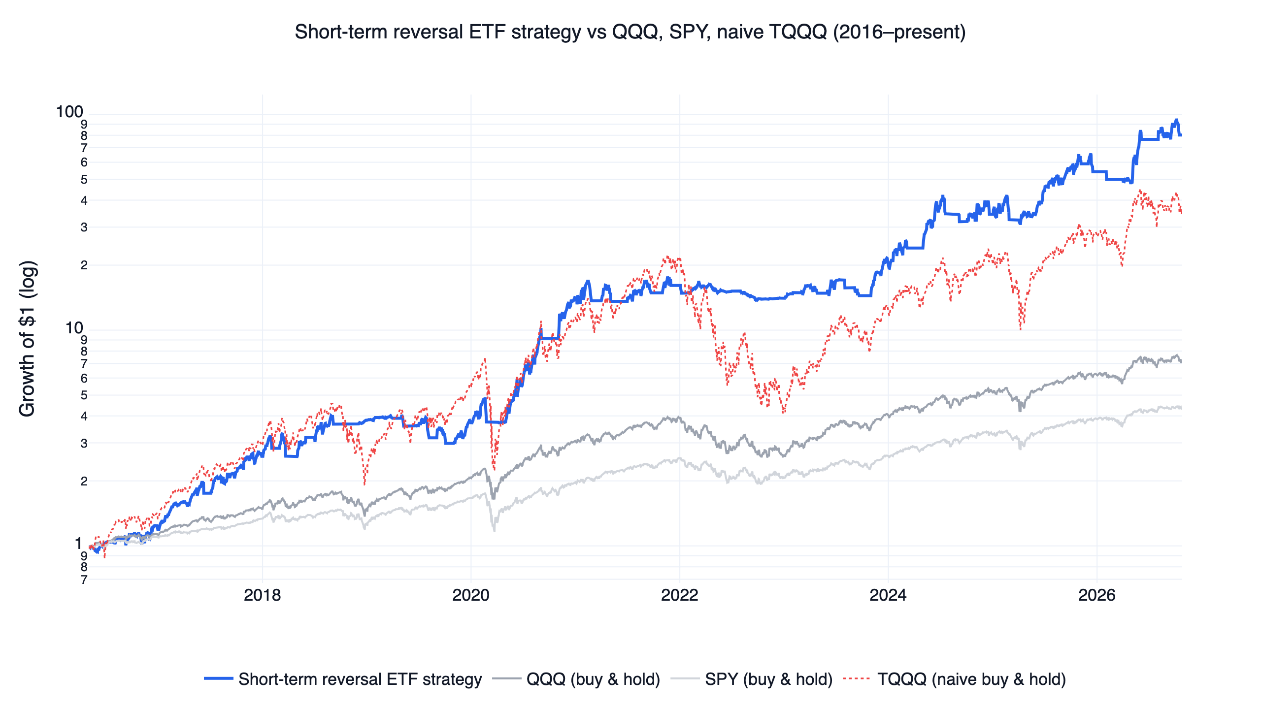
Our other stock-level studies on S&P 500 members came out the same way. The golden cross stocks backtest returned 11.5% a year with a Sharpe ratio of 0.72 over 2017 to 2026, and the 52-week high stocks backtest lost to QQQ in all 63 settings. Those are trend rules with turnover of about 2.5 and 13 times a year. The mean reversion rule here turned over 33 times: before costs it earned more than either, and at 0.1% per side its Sharpe ratio of 0.43 fell below the golden cross rule's 0.68. A different, regime-filtered version of short-term mean reversion on leveraged ETFs is in our short-term mean reversion strategy.
The code
This is the S&P 500 %B mean reversion rule. On data through 2026-11-05 it prints a daily Sharpe of about 0.75; the last digit can move as FinLab revises its data. research.py also keeps one share class per company and runs the other three rules, all 36 settings and the six checks.
Show Code
import finlab
from finlab import data
from finlab.backtest import sim

finlab.login()
data.set_market("us")

close = data.get("us_price:adj_close")
members = data.get("us_index_constituents:sp500").astype(bool)

# Keep tickers in both tables and line the members up with trading days
tickers = members.columns.intersection(close.columns)
close = close[tickers]
members = members[tickers].reindex(close.index, method="ffill").fillna(False).astype(bool)

# 20-day Bollinger Bands, 2 standard deviations either side
middle = close.rolling(20).mean()
lower = middle - 2 * close.rolling(20).std(ddof=0)

# Buy a member that closes below its lower band; sell back at the middle band
buy = (close < lower) & members
sell = (close >= middle) | ~members
position = buy.hold_until(sell).loc["2016-09-01":]

# Equal weight, at most 5% in a stock, traded at the next open
report = sim(position.loc[:, position.any()], position_limit=0.05, trade_at_price="open",
             market="us", upload=False)

returns = report.creturn.pct_change().dropna()
print("Daily Sharpe:", round(returns.mean() / returns.std() * 252 ** 0.5, 2))
Install the FinLab skill for your AI agent
You do not need to write this yourself. Install the FinLab skill in Claude Code, Codex or Gemini CLI with one command:
Show Code
npx skills add koreal6803/finlab-ai --skill finlab -g -yThen ask your agent in plain language, for example "run the Bollinger Band squeeze on Nasdaq 100 members" or "add a 5-day time stop to the lower band rule and charge 0.05% per side". The agent setup page has the details, and FinLab Studio runs the same research in a browser.
Backtest method and limits
| Item | How it was handled |
|---|---|
| Window | 2016-09-01 to 2026-11-05. FinLab's US prices start in January 2016, and the first months warm up the 126-day BandWidth |
| Universe | Each day's S&P 500 members, one share class per company. Members without a FinLab price are skipped |
| Liquidity | No filter beyond index membership. Capacity is not estimated |
| Turnover | 33 times a year for mean reversion and 21 for the squeeze, one way on target weights; 3.9 and 1.6 for the QQQ rules |
| Signals | Bands use closes up to the signal day, with no later data (look-ahead bias control) |
| Weights | Equal, capped at 5% a stock, re-equalised on days the list changes; cash earns nothing |
| Execution | Signal at a close, traded at the next day's open, on adjusted prices |
| Cost | finlab sim() default US cost of zero, plus a rerun at 0.1% per side. Slippage is not estimated separately |
| Taxes | None |
| Sample | Whole window in-sample. The halves only check stability; no out-of-sample test was run |
What this result does and does not say
Within this window and these rules, buying S&P 500 stocks at the lower band earned a little more per unit of risk than holding them all at equal weight, before costs, and less after realistic costs. Nothing here beat QQQ, which had an unusually strong decade. The test covers large, liquid US stocks only; small caps, other markets or added filters such as a trend condition may behave differently, and each would need its own test.
For a first strategy in Python, the US stock backtest tutorial walks through the steps, and the US strategy comparison collects the rest of our work.
FAQ
What is the best Bollinger Bands strategy?
None of the four we tested beat QQQ. The strongest was buying S&P 500 stocks that close below the lower band and selling at the middle band: 14.3% a year and a Sharpe ratio of 0.75 before costs, against 0.89 for QQQ.
Does buying at the lower Bollinger Band work?
On individual S&P 500 stocks it edged the equal-weight index before costs, 0.75 against 0.70, and 69.1% of 22,631 trades made money. With 0.1% per side its return fell to 6.9% a year. On QQQ it returned 3.3% a year.
What is a Bollinger Band squeeze?
A squeeze is BandWidth, the gap between the bands relative to the middle band, at its lowest in about six months. We bought S&P 500 stocks that broke above the upper band within 20 days of a squeeze: 8.0% a year, a -16.8% drawdown and a Sharpe ratio of 0.70, the same as RSP.
Are 20 days and 2 standard deviations the best settings?
Not here, and no setting stood out. For mean reversion, 15-day bands scored 0.76 to 0.77 and 25-day bands 0.59 to 0.67. For the squeeze, 25 days and k = 2 scored 0.78. All were below QQQ's 0.89.
Do Bollinger Bands work on QQQ?
Not as timing tools in this test. Both QQQ rules sat in cash most of the time and scored 0.29 and 0.15, while holding 18.2% of the account in QQQ every day scored 0.90. We did not test SPY.
How much do trading costs matter for Bollinger Band strategies?
A lot for the stock rules. Mean reversion traded 33 times its portfolio a year, so 0.1% per side cut its return from 14.3% to 6.9% and its Sharpe ratio from 0.75 to 0.43.
Can I rerun this?
Yes. Install the FinLab skill through the AI-assisted setup, download research.py below and run python research.py.
Reproduce it yourself
- research.py: the four rules, the 36 settings, both halves, the cost runs and the six checks.
- data.csv: daily equity curves of the four rules at their original settings, plus QQQ, SPY and RSP.
- metrics.json: the statistics behind this article, including trades, holdings and calendar-year returns.
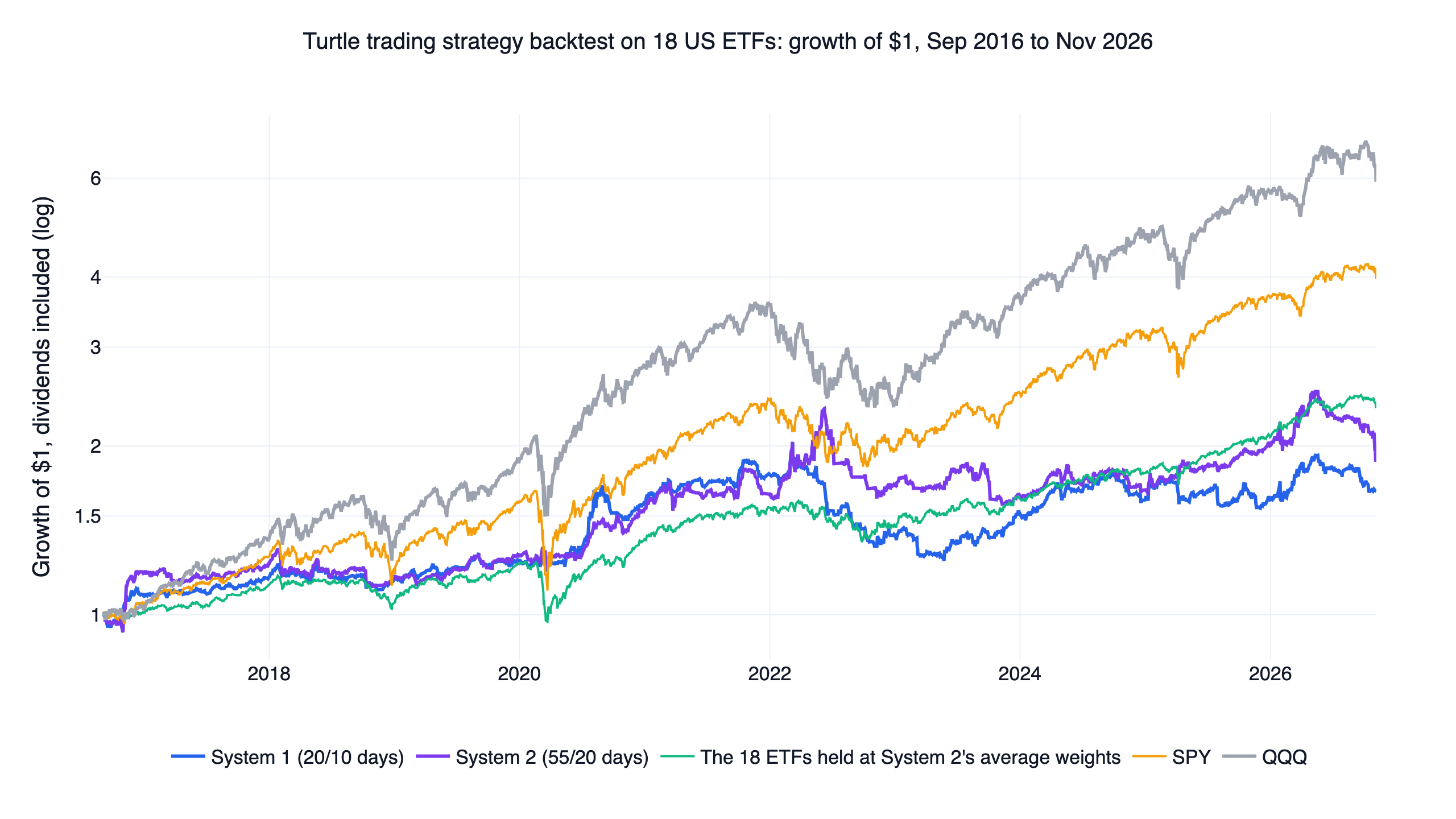
New research is on the FinLab blog, the team is on the about page, and examples are on use cases. A trend-following rule with a channel breakout is in the Turtle trading strategy backtest.
Disclaimer: this article is for education only and does not constitute investment advice. Past performance does not guarantee future results, and investing involves risk. All results are in-sample, and the two halves were not validated out of sample.
Last updated: 2026-11 | Backtest window: 2016-09 to 2026-11 | Data through 2026-11-05, run 2026-11-07 | Benchmark: QQQ total return | Author: FinLab Quant Research (reviewed by a quantitative researcher)
FinLab AI
Want to build your own strategy?
Describe your stock-picking ideas in natural language. AI automatically validates, backtests, and gives you answers
Start Free