Run this strategy
Copy the prompt to reproduce the evidence above with the article’s data, assumptions, and risk checks.
Tell your AI:
Help me set up FinLab and rerun this US price-to-book backtest. Please read: https://finlab.finance/en/setup?relatedUrl=/en/blog/us-stock-backtest-price-to-book-strategy
Price-to-book is the oldest value screen in the book, and in some markets it sorts stocks. In FinLab's Taiwan-market study, the cheapest fifth of the market by P/B compounded at 14.17% a year from 2010 to 2026 and the most expensive fifth at 7.57%, with every quintile in between falling neatly into order over the full period, though the order has reversed since 2024. This article takes that exact template, moves it to US stocks, and runs it through a complete US stock backtest in Python with finlab: data loading, factor construction, cross-sectional tests, and a tradable portfolio.
Over March 2016 to October 2026 the answer is clear. The monthly Rank IC of book-to-price averaged -0.0091 (t = -0.67), statistically indistinguishable from zero. The cheapest decile earned 1.07 percentage points a year less than the most expensive one. A tradable portfolio of the 50 cheapest stocks compounded at 10.38% with a -48.1% maximum drawdown, against 20.47% for QQQ and 15.40% for SPY, both with dividends reinvested. It also fails all three robustness checks further down: neighbouring parameters, two halves of the sample, and trading costs.
So the page does two jobs. It is a working template for any US stock backtest you want to run, with every step in readable code, and it is a documented failure of a factor that many value investors still treat as a default. If you only want strategies that held up under the same tests, skip to US strategies that pass the same checks.
The numbers at a glance
| Portfolio | Window | CAGR | Daily Sharpe | Max drawdown | Total return |
|---|---|---|---|---|---|
| Cheapest-B/P 50 stocks (monthly rebalance, 46 held on average) | 2016-03 to 2026-10 | 10.38% | 0.53 | -48.1% | +186.5% |
| QQQ (total return) | same | 20.47% | 0.95 | -35.1% | +627.3% |
| SPY (total return) | same | 15.40% | 0.90 | -33.7% | +359.7% |
| Factor test | Value | Reading |
|---|---|---|
| Mean monthly Rank IC of B/P | -0.0091 (t = -0.67) | No different from zero |
| Months with positive IC | 46.1% | Worse than a coin flip |
| D10 (cheapest) minus D1 (most expensive), annualized | -1.07% | The cheapest decile lost |
| Portfolio monthly Sharpe | 0.56 | 24.4% annualized volatility |
| Robustness checks | 0 of 9 parameter sets beat QQQ; both halves lose; still loses with 0.1% costs | Fails all three |
All figures come from a finlab backtest on data through 2026-10-26. QQQ and SPY are buy-and-hold on dividend-adjusted prices, rebased to the same start date as the portfolio.
Install the FinLab skill for your AI agent
You do not have to type the code below by hand. FinLab ships as a skill that AI coding agents load when they need it, so you can describe a test in plain English, such as "rerun the book-to-price deciles on the top 600 stocks and compare against QQQ", and let the agent write and run the finlab code. One command installs it:
Show Code
npx skills add https://github.com/koreal6803/finlab-ai --skill finlabThe skill works with Claude Code, Codex, and Gemini CLI; the agent setup page lists the steps for each one. If you would rather not install anything locally, FinLab Studio runs the same research in the browser. The AI-assisted setup flow handles login and walks you through a first backtest.
A US stock backtest in Python: the full finlab workflow
finlab uses the same syntax for every market. After data.set_market("us"), data.get(), the FinlabDataFrame methods, and the sim() backtester behave exactly as they do elsewhere. This block is the core of every number in the article, one action per line:
Show Code
import finlab
from finlab import data
from finlab.backtest import sim

finlab.login()          # finlab guides you through login when data is first requested
data.set_market("us")   # switch to US data

# 1. Load prices, volume and fundamentals
close = data.get("us_price:adj_close")   # adjusted close: returns and B/P
raw_close = data.get("us_price:close")   # unadjusted close: dollar volume and price floor
volume = data.get("us_price:volume")
eps = data.get("us_income_statement:eps_diluted")
net_income = data.get("us_income_statement:net_income")
equity = data.get("us_balance_sheet:total_stockholders_equity")

# 2. Liquid universe: top 500 by 60-day average dollar volume
# Volume is not split-adjusted, so dollar volume uses the unadjusted close
dollar_volume = (raw_close * volume).rolling(60, min_periods=20).mean()
# The downloadable script also drops names with an extreme one-day move in the past year
universe = (
    dollar_volume.is_largest(500)
    & (raw_close > 10)
    & (dollar_volume > 10_000_000)
)

# 3. Build book-to-price
# There is no shares-outstanding field, so derive shares from TTM net income / TTM diluted EPS
ttm_eps = eps.rolling(4).sum()
ttm_net_income = net_income.rolling(4).sum()
shares = ttm_net_income / ttm_eps

book_per_share = equity / shares
bp = book_per_share / close     # higher B/P = cheaper

# Derived share counts blow up when EPS is near zero, so guard the edge cases
valid = (ttm_eps.abs() > 0.05) & (equity > 0) & (shares > 0) & universe
bp = bp[valid]

# 4. Cheapest quintile, then the 50 highest B/P names, rebalanced monthly
cheapest_quintile = bp.rank(axis=1, pct=True) > 0.8
position = bp[cheapest_quintile].rank(axis=1, ascending=False) <= 50

# 5. Backtest with zero commission and tax (US zero-commission brokers)
report = sim(
    position,
    resample="M",
    fee_ratio=0,
    tax_ratio=0,
    position_limit=0.05,
    upload=False,
)
report.display()
Four details matter more in US data than they look:
- Dataset keys. US stock prices live under
us_price:, statements underus_income_statement:andus_balance_sheet:, and ETF total-return prices underus_fund_price:adj_close, which is where the QQQ and SPY benchmarks come from. - Shares have to be derived. With no direct shares-outstanding field, the standard trick is TTM net income divided by TTM diluted EPS. When EPS is close to zero this produces absurd share counts, so the code requires
|TTM EPS| > 0.05and positive equity. Skip that guard and a handful of outliers dominate the ranking. - The universe is the first quality gate. The US market lists far more penny stocks and broken tickers than most. This backtest uses a rolling universe of the top 500 stocks by 60-day dollar volume, with a 10M daily dollar-volume floor, and a one-year exclusion after any single-day move of 50% or more. FinLab's
us_price:volumeis not split-adjusted whileadj_closeis, so multiplying the two overstates a stock's dollar volume before a reverse split by the split ratio, by as much as about 100,000x for some microcaps. That let tiny reverse-split names into the top 500 and past the $10 floor, so dollar volume and the price floor now use the unadjusted close (us_price:close), and returns still use the adjusted close. - Statements are aligned to filing dates. finlab's US fundamentals are point-in-time by SEC filing date, so each month's ranking only uses numbers that had been published by then. That removes the most common source of look-ahead bias in fundamental backtests.
Factor analysis, layer 1: does book-to-price sort US stocks?
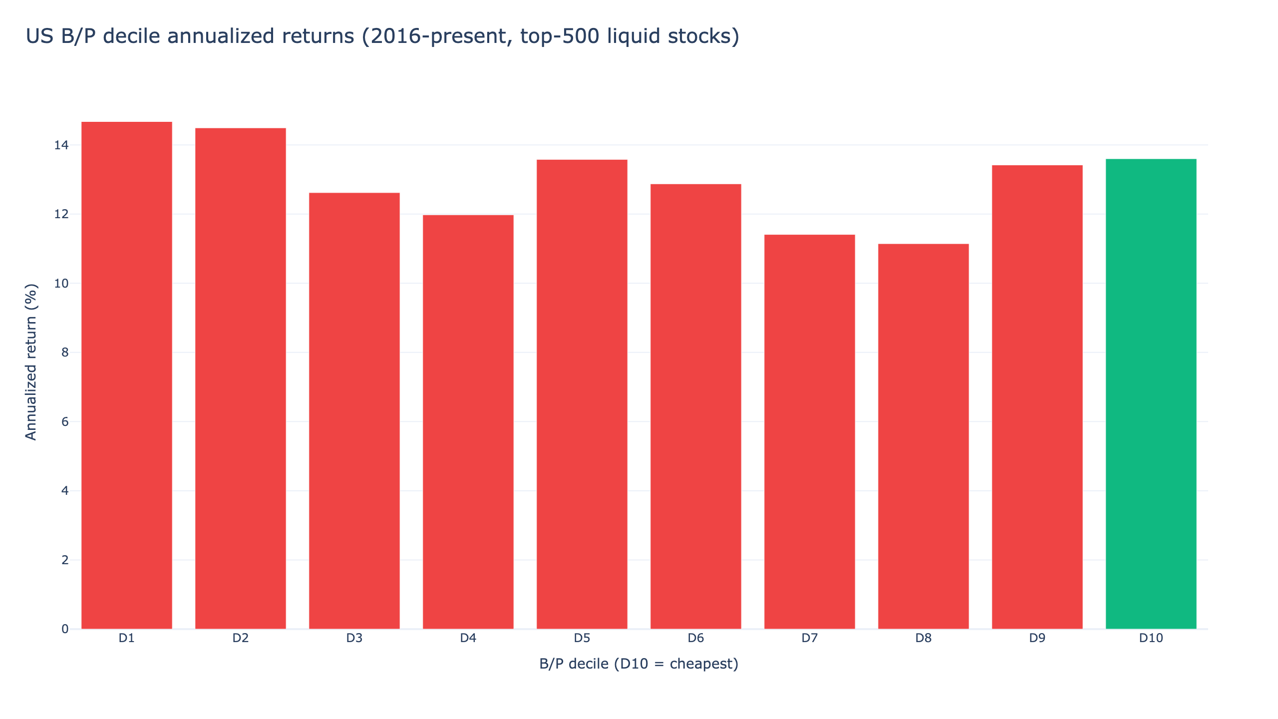
Before building a portfolio, test whether the signal ranks stocks at all. Each month-end, the liquid universe is split into ten deciles by B/P, and the next month's equal-weighted return of each decile is recorded. If cheapness paid in US stocks, the chart at the top of this page would rise from D1 (most expensive) to D10 (cheapest). It does not. Over the full window D1 earned 14.67% a year and D10 13.60%, and the middle deciles jump around with no order: D8 is the weakest at 11.14%, while D5 and D9 sit close to D10. The long-short spread, D10 minus D1, is -1.07% a year.
The second test is the monthly Rank IC: the rank correlation between each stock's B/P at month-end and its return over the following month, computed across the whole universe. A useful factor shows a mean IC reliably above zero. This one averaged -0.0091 with a t-statistic of -0.67, and only 46.1% of months were positive.
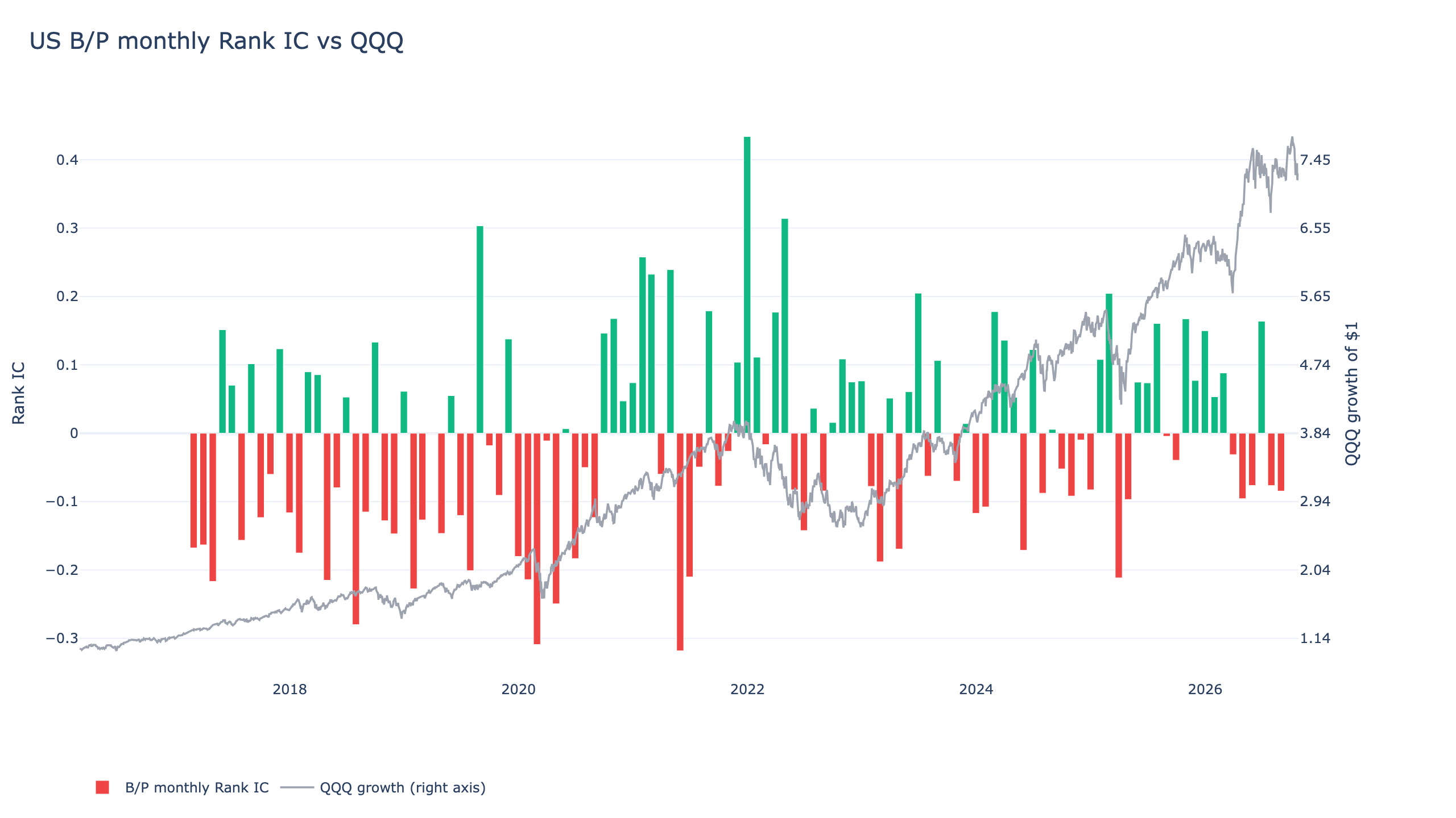
The right axis plots QQQ's cumulative return as market context. Whether growth stocks were running or correcting, the IC flips sign from month to month around zero. There is no regime in this chart in which B/P reliably pointed the right way.
Factor analysis, layer 2: the tradable portfolio vs QQQ and SPY
Deciles are a description, not a portfolio. The tradable version takes the cheapest B/P quintile, keeps the 50 names with the highest B/P, weights them equally with a 5% cap per stock, and rebalances monthly. On average it held 46 stocks. All three lines below are rebased to the same start date.
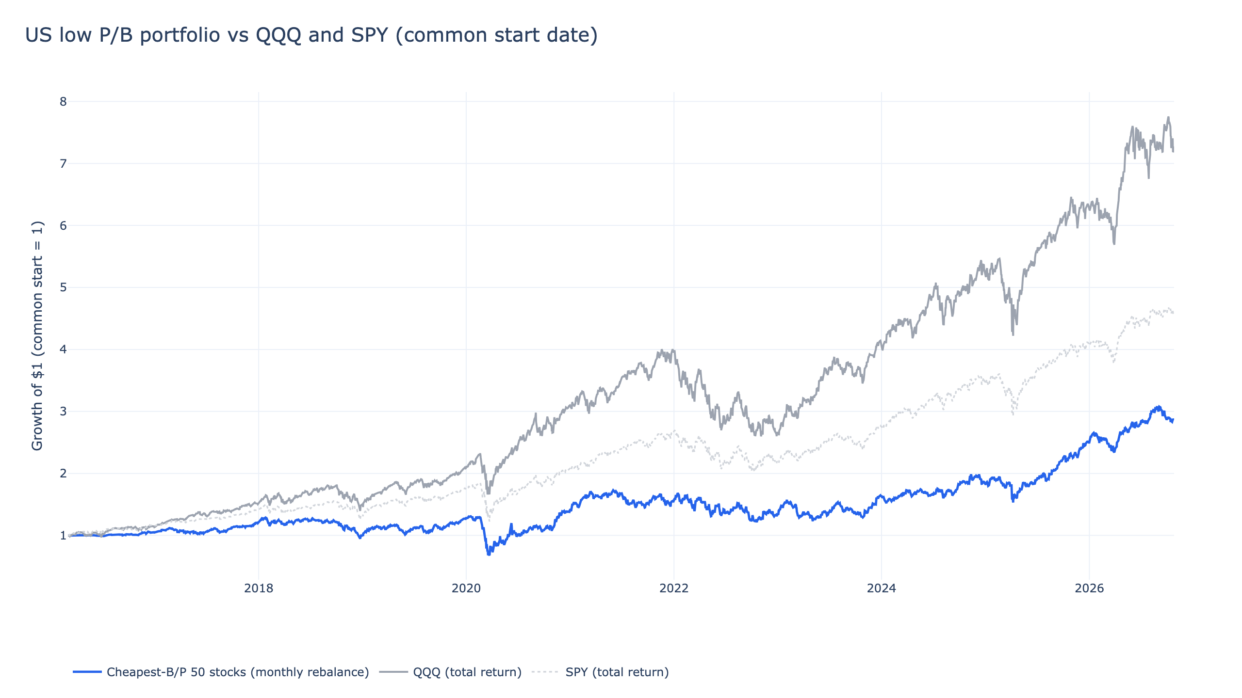
Over ten and a half years the portfolio returned +186.5% in total, or 10.38% a year. SPY returned +359.7% and QQQ +627.3% over the same dates. The risk side is worse: 24.4% annualized volatility against QQQ's 22.1%, and a -48.1% maximum drawdown, 13 to 14 percentage points deeper than either index ETF. The portfolio took on more volatility than QQQ for about half of its annual return and less than a third of its total return.
The interactive report has the full equity curve, drawdowns, holdings, and trade list:
To rerun it or change the settings, strategy.py produces every number and chart in this article, and metrics.json stores the results in machine-readable form.
Research window vs out-of-sample: the ranking flips
The full-window average hides the most interesting fact: the factor changed direction during the sample. Splitting the deciles into a research window (2016 to the end of 2021) and an out-of-sample window (2022 onward):
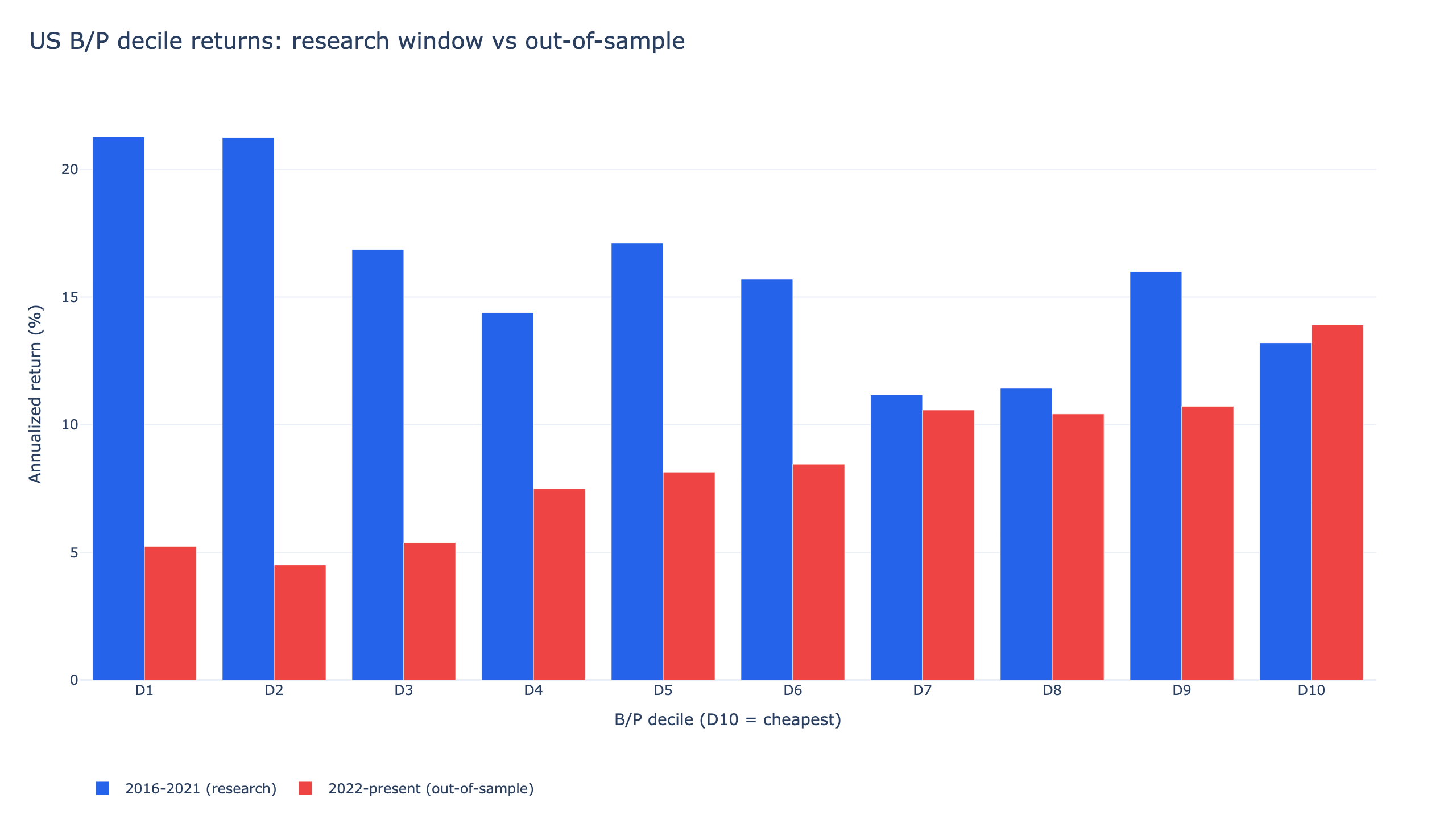
- Research window, 2016-2021. D1, the most expensive and most growth-heavy decile, led at 21.29% a year, with D2 at 21.25%. D10, the cheapest, earned 13.22%. Buying expensive stocks was the right call.
- Out-of-sample, 2022 onward. The order reversed. D1 fell to 5.25% and D2 to 4.51%, while D10 led at 13.91%, and returns rose roughly step by step from D2 to D10. The rate-hiking environment from 2022 put cheap stocks back in front.
The -1.07% full-window spread is what is left when two opposite regimes cancel. Anyone researching at the end of 2021 would have concluded "buy growth"; anyone researching at the end of 2022 would have concluded "value is back". In US stocks the direction of a single value factor is itself a bet, and a backtest cannot settle it. Even in the out-of-sample years, when the ranking favoured cheap stocks, the tradable portfolio still trailed QQQ, which the next section quantifies.
Robustness checks: neighbouring parameters, two halves, trading costs
"Beats QQQ" in this section means a higher daily Sharpe ratio (mean daily return divided by its standard deviation, annualized with √252, no risk-free rate) than buying and holding QQQ with dividends over exactly the same dates. Because each comparison uses the strategy's own dates, QQQ's figure moves slightly between tests.
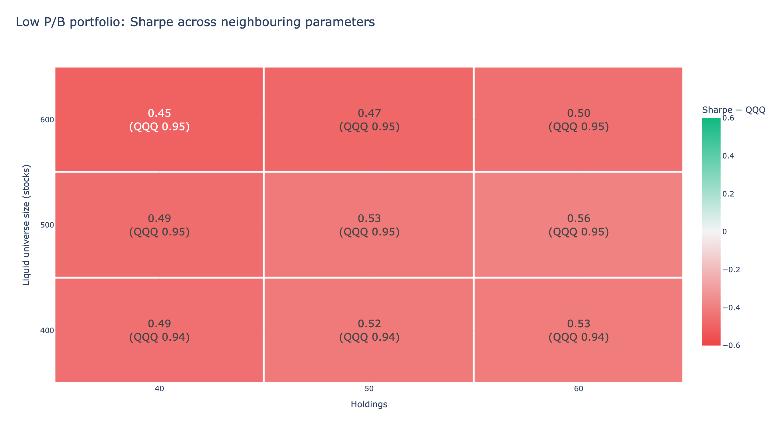
Neighbouring parameters. The two main parameters were each moved one step either side of the original: the size of the liquid universe (top 400, 500, or 600 stocks by dollar volume) and the number of holdings (40, 50, or 60). The pass mark is at least 7 of the 9 combinations beating QQQ. None of the 9 did. The original setting (top 500, 50 holdings) scores 0.53 against QQQ's 0.95; across the grid the portfolio ranges from 0.45 to 0.56 while QQQ sits at 0.94 to 0.95. More holdings help slightly, but the best cell reaches only about 60% of QQQ's Sharpe.
Two halves. Cutting the backtest in half by trading days:
| Half | Dates | Portfolio daily Sharpe | QQQ daily Sharpe |
|---|---|---|---|
| First half | 2016-03-01 to 2021-06-25 | 0.51 | 1.18 |
| Second half | 2021-06-25 to 2026-10-26 | 0.55 | 0.73 |
Both halves lose. The second half includes the out-of-sample years in which cheap stocks beat expensive ones, and the gap narrows, but the portfolio still trails QQQ by 0.18. A factor can rank stocks correctly against each other without producing a portfolio that beats the index.
Trading costs. finlab's US-market default charges zero commission and zero tax, matching zero-commission brokers, so the headline run carries no trading cost at all. Charging 0.1% on every buy and every sell (fee_ratio=0.001) as a stand-in for spread and slippage, CAGR drops from 10.38% to 9.9% and the daily Sharpe to 0.51, against QQQ's 0.97 over the same dates. The portfolio was already behind, and costs widen the gap.
Verdict: fails all three checks (0 of 9 neighbouring settings, both halves, and the cost test). For a reader, that means this portfolio should not be used as an investment method, and changing the universe size or the number of holdings does not change the outcome. Its value is as a worked example of a factor failing its tests. To reproduce every number in this section, run python strategy.py --validate with the downloadable script.
Why price-to-book works in Taiwan but not in the US
Put the two studies side by side, built with the same tools and the same method, and the contrast is clean. In Taiwan, over the full period, P/B quintile returns fall in strict order and the cheapest quintile earns about 1.9 times the most expensive one. In the US, the deciles are scrambled, the cheapest decile trails the most expensive, and the IC is statistically zero. Three explanations fit.
The factor has been priced. Fama & French (1992) established book-to-market as one of the strongest explanators of US cross-sectional returns, building on early evidence such as Rosenberg, Reid & Lanstein (1985). In the three decades since, the US has become the most heavily researched and arbitraged equity market in the world. McLean & Pontiff (2016) measured what that does: across 97 published predictors, US returns to the anomaly portfolios fell substantially after publication, consistent with investors trading on the research. A market with more retail participation and thinner quantitative coverage, such as Taiwan, leaves more of a simple valuation signal intact.
Book value measures the wrong thing for today's large caps. The top 500 US stocks by liquidity are dominated by technology and services companies whose main assets, such as research, software, and brands, are expensed rather than capitalized. Book equity misses most of what these firms own. Arnott, Harvey, Kalesnik & Linnainmaa (2021) show that the treatment of intangibles matters a great deal for book-based value measures, and also argue that reports of value's death are exaggerated, with much of its slump explained by widening valuation spreads. The out-of-sample reversal here, with D10 leading after 2022, fits that "damaged but not dead" description: some mean reversion is left, but not enough to build a portfolio that beats the index.
Value alone is fragile anywhere. Asness, Frazzini, Israel & Moskowitz (2015) stress that a stand-alone value factor is volatile, suffers deep drawdowns, and can underperform for a decade, which is why practitioners almost always combine it with quality or momentum. The Taiwan result agrees: the ranking works there over the full period, though the order has reversed since 2024, and all five quintiles still trail the Taiwan 50 ETF (0050) with dividends, which compounded at 17.24%.
The practical rule: the template of a strategy travels between markets, since the syntax and the workflow are identical, but the factor and its parameters do not. Every factor has to be re-validated in the market where you intend to trade it.
What the 2023 version of this article got wrong
The first version of this article, published in Chinese in July 2023, presented this low-P/B strategy as an example from FinLab's online strategy lab and concluded from a 2016 to mid-2023 backtest screen that it had beaten the S&P 500 over seven years and fallen less in the 2020 COVID sell-off. Rerun over the full March 2016 to October 2026 window, neither claim holds: 10.38% a year against 15.40% for SPY with dividends, and a -48.1% maximum drawdown against SPY's -33.7%.
The same backtest contradicts both claims over the window the original version covered, too. From 2016-03-01 to 2023-06-30 the portfolio returned +37.1% cumulatively, against +125.0% for the S&P 500 price index. Its worst drawdown of the entire decade came in the COVID crash itself: -48.1% from the January 17, 2020 peak to the March 23 low, while the S&P 500 index fell 32.8% over the same dates. Across the nine calendar years from 2016 (starting in March) to 2024, the portfolio beat the S&P 500 index only once, in 2022, when it fell 14.4% against the index's 19.4%, the year just before the 2023 review, when the impression of cheap stocks as a defensive holding was freshest. The gap between the 2023 screen and today most likely comes from the data version and stock universe the online lab used at the time; it cannot be attributed item by item, which is why the full script and metrics file are published. The last two years have been better for the portfolio: +35.7% in 2025 and +15.3% in 2026 through October 26, ahead of the S&P 500 index's 16.4% and 12.1%. Over the full window its CAGR and Sharpe still trail both SPY and QQQ.
US strategies that pass the same checks
The useful follow-up question is which US strategies did hold up. We ran a family of US systems on the same data engine and universe method, and the six below pass the same three robustness checks in this October 2026 update. Each article includes the full code, a factor or signal analysis, and an out-of-sample split; their performance figures and windows are in the articles themselves.
| Strategy | Signal | What it actually holds |
|---|---|---|
| Momentum | Breadth of 12-1 momentum leaders plus the QQQ trend | Leveraged growth ETFs, or defensive ETFs |
| Quality value (free-cash-flow version) | Breadth of free-cash-flow and balance-sheet strength | Leveraged growth ETFs, or defensive ETFs |
| Earnings surprise | Breadth of positive earnings surprises plus the market trend | Leveraged growth ETFs, or defensive ETFs |
| Low volatility | QQQ regime filter that avoids high-volatility periods | One 2x index ETF, or a defensive ETF |
| Short-term mean reversion | In a QQQ uptrend, the 3x ETF that lagged over 3 days | One 3x growth ETF, or a defensive ETF |
| ETF rotation | QQQ 200-day average plus 126-day return as a risk switch | 2x or 3x ETFs, or a defensive sleeve |
These are a different kind of strategy from the low-P/B portfolio. This article holds individual stocks; the six above use factors as timing signals and hold leveraged or defensive ETFs. Leveraged ETFs reset daily, so their returns depend on the path the market takes and decay in volatile, sideways markets; held blindly, they have suffered drawdowns of well over 60%. Each article covers those risks in full.
The quality-value article is the closest relative of this one. It measures value through cash flow, combines it with balance-sheet quality, tests the factors at the stock level with deciles and Rank IC, and then turns them into a market-breadth signal that decides when to hold leveraged ETFs. The version that passes the checks is that timing version, and it holds ETFs, not the screened stocks. That matches the research above: value needs a better measure than book equity, and it should not be used on its own. The US quant trading strategies overview compares the whole family of ten on the same data.
Backtest method and limits
| Item | This backtest |
|---|---|
| Window | 2016-03-01 to 2026-10-26; research window 2016 to end-2021, out-of-sample 2022 onward; the robustness check also splits the sample in half at 2021-06-25 |
| Data and version | finlab 2.2.20, data through 2026-10-26. In October 2026 FinLab added missing dividends to US adjusted prices and fixed split and spin-off adjustments, so historical figures differ from earlier versions of this study |
| Universe | Rolling top 500 by 60-day average dollar volume, price of at least 10M, and a one-year exclusion after any single-day move of 50% or more. Dollar volume and the price floor use the unadjusted close (us_price:close); with adjusted close, reverse-split microcaps would fill the universe and distort every result. The numbers changed with the data corrections and the conclusion stands |
| Survivorship | The universe is rebuilt point-in-time from rolling price and volume alone, with no current-only fields such as today's market cap or index membership. Whether every delisted US stock is present in the price history was not separately audited |
| Factor | B/P = book value per share / adjusted close; shares derived as TTM net income / TTM diluted EPS, with |TTM EPS| > 0.05, positive equity, and positive shares required |
| Look-ahead bias | Statements aligned to filing dates by finlab's data layer (point-in-time); returns from adjusted closes |
| Portfolio rule | Cheapest B/P quintile, top 50 by B/P, equal weight, 5% position limit, monthly rebalance; 46 holdings on average |
| Transaction costs | The headline run uses finlab's US default of zero commission and zero tax (zero-commission brokers), so it carries no trading cost. The cost check charges 0.1% per buy and per sell for spread and slippage: CAGR 9.9% instead of 10.38%, daily Sharpe 0.51 against QQQ's 0.97 |
| Turnover and capacity | Not estimated |
| Benchmarks | QQQ and SPY buy-and-hold on dividend-adjusted prices (us_fund_price:adj_close), rebased to the portfolio's start date |
| Deciles and IC | Month-end B/P deciles across the universe, next-month equal-weighted returns and Rank IC; descriptive statistics with no trading costs |
| Robustness | Neighbouring parameters (9 sets), two halves, and 0.1% per-side costs, each compared with QQQ on daily Sharpe; fails all three |
| Statistical limits | About ten years of monthly data is short relative to value cycles that can last five to ten years; the direction flips between sub-periods, so the full-window average says little about the future |
FAQ
How do I backtest US stocks in Python?
Install finlab, call data.set_market("us"), and load US datasets with data.get(); the backtest itself is a single sim() call on a boolean or weight table. The code block above is a complete minimal workflow. The fastest route is to install the FinLab skill for your AI agent and ask it to build the test for you through the AI-assisted setup flow.
Does the price-to-book ratio still work in US stocks? Not as a stand-alone factor in the liquid US universe over 2016-2026. The mean monthly Rank IC was -0.0091, the cheapest decile trailed the most expensive, and a 50-stock low-P/B portfolio compounded at 10.38% against 20.47% for QQQ. The ranking did favour cheap stocks after 2022, but even then the portfolio trailed QQQ on Sharpe.
Why rank by book-to-price rather than price-to-book? Book-to-price is the same information inverted, with higher meaning cheaper. It behaves better numerically: P/B explodes as book value approaches zero and flips sign when book turns negative, while B/P simply moves toward zero, so it ranks cleanly. Companies with negative equity are excluded here rather than ranked.
Would different parameters fix it? No. All nine combinations of universe size (top 400, 500, 600) and holdings (40, 50, 60) scored a daily Sharpe between 0.45 and 0.56, against 0.94 to 0.95 for QQQ.
Can a strategy from another market be moved to US stocks? The workflow can; the factor cannot be assumed to survive. This article is a direct counterexample: the same P/B template sorts Taiwan stocks over the full period, though the order has reversed since 2024, and does nothing in the US. Before trading any ported strategy, rerun the deciles, the IC, a sub-period split, and the three robustness checks.
How much do trading costs and slippage matter here? US commissions are zero at most brokers, so the main cost is the bid-ask spread and market impact. Charging 0.1% per buy and per sell lowered CAGR from 10.38% to 9.9%. Larger accounts face more impact, depending on order size relative to each stock's daily volume; capacity was not estimated.
Reproduce it yourself
- strategy.py: the full script.
python strategy.pyrebuilds the deciles, IC, portfolio, and charts;python strategy.py --validateruns the three robustness checks. - metrics.json: every metric in this article.
For a market-timing study rather than a stock factor, see buying US stocks after VIX spikes. More research is on the FinLab blog, metric definitions are in the glossary, and the use cases and about page show who builds with finlab.
Last updated: 2026-10 | Backtest window: 2016-03 to 2026-10 | Benchmark: QQQ total return | Author: FinLab Quant Research (reviewed by a quantitative researcher)
Investing involves risk, and past performance does not represent future results. This article documents a factor that failed its tests: the low price-to-book portfolio trailed both index ETFs and failed all three robustness checks, so do not use it as an investment method. Other strategy results mentioned are historical backtests and do not guarantee future returns. This content is for educational purposes only and is not investment advice.
FinLab AI
Want to build your own strategy?
Describe your stock-picking ideas in natural language. AI automatically validates, backtests, and gives you answers
Start Free