Run this strategy
Copy the prompt to reproduce the evidence above with the article’s data, assumptions, and risk checks.
Tell your AI:
Set up FinLab and add a 200-day moving average filter on QQQ to my US strategy. Please read: https://finlab.finance/en/setup?relatedUrl=/en/blog/200-day-moving-average-market-filter
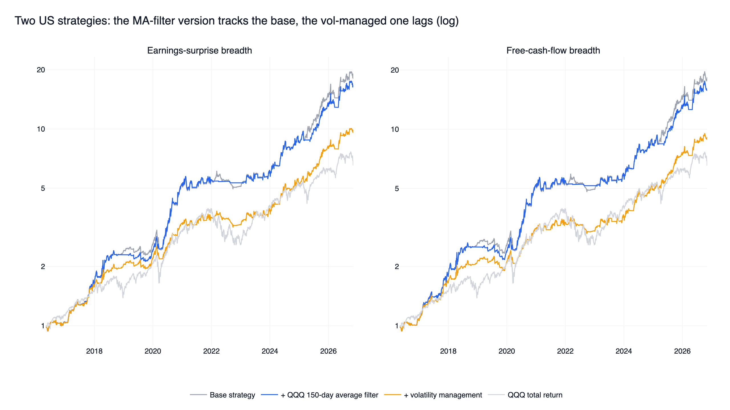
Does a 200-day moving average market filter make a good strategy better? We took the two US strategies on our strategy pages and added the classic trend rule on top: sell everything when QQQ closes below its moving average (100, 150 or 200 days, with a 0 to 4% buffer), buy back when it closes above. From May 2016 to November 2026 the filter cut the maximum drawdown of the earnings-surprise strategy from -21.1% to -15.3% and moved its daily Sharpe ratio from 1.46 to 1.48, but its Sharpe ratio above T-bills beat the base in only 4 of 9 settings. For the free-cash-flow strategy the Sharpe ratio fell from 1.47 to 1.45. The weekly returns of both filtered versions correlated 0.97 with the originals, so they are the same strategies with slightly less exposure. Neither passed the conditions we wrote down before the test, and monthly volatility management did worse.
The reason is that both strategies already use the same signal. They only go risk-on when QQQ is above its 200-day average with positive six-month momentum, and otherwise hold the strongest of IEF, GLD and SHY. On the 15.3% of days the filter sat in cash, they earned 5.5% and 9.9% a year, with Sharpe ratios of 0.40 and 0.74 against 1.61 and 1.58 on the other days. QQQ itself earned 18.2% a year on those days, with twice its usual volatility. A moving average filter helps only if the strategy underneath earns little or loses money while the market is below its average.
200-day moving average filter results at a glance
| Earnings-surprise breadth | Free-cash-flow breadth | QQQ total return | |
|---|---|---|---|
| Base strategy: CAGR / daily Sharpe / max drawdown | 31.6% / 1.46 / -21.1% | 31.8% / 1.47 / -21.1% | 19.7% / 0.92 / -35.1% |
| With QQQ 150-day filter, 2% buffer | 30.7% / 1.48 / -15.3% | 30.0% / 1.45 / -18.4% | |
| With volatility management (63 days, 1.0) | 23.9% / 1.43 / -17.7% | 23.4% / 1.42 / -17.7% | |
| Sharpe above T-bills: base / filter / vol | 1.35 / 1.36 / 1.29 | 1.36 / 1.33 / 1.28 | 0.82 |
| Settings beating the base (filter / vol) | 4 of 9 / 1 of 9 | 2 of 9 / 2 of 9 | |
| Weekly correlation with the base (filter / vol) | 0.97 / 0.97 | 0.97 / 0.97 | |
| Passed | No | No |
What a 200-day moving average market filter does
A moving average is the average closing price of the last N trading days. The 200-day moving average covers about ten months, and "QQQ is below its 200-day" is one of the most common ways to say a market is in a downtrend. As a market filter it does not pick stocks; it decides whether the whole portfolio is invested. When the index closes below its average, everything is sold; when it closes back above, the strategy's current holdings are bought back.
Faber (2007) made the rule popular with a 10-month average on US stocks and other asset classes: returns close to buy-and-hold with much smaller drawdowns. We used two lines. The filter goes to cash when QQQ (dividends reinvested) closes below its N-day average times (1 - buffer), returns when QQQ closes at or above the average, and between the two lines it keeps the previous day's state, so it does not flip every time the index touches the line. The original setting is 150 days with a 2% buffer, the middle of a 3 x 3 grid of 100, 150 and 200 days by 0%, 2% and 4%.
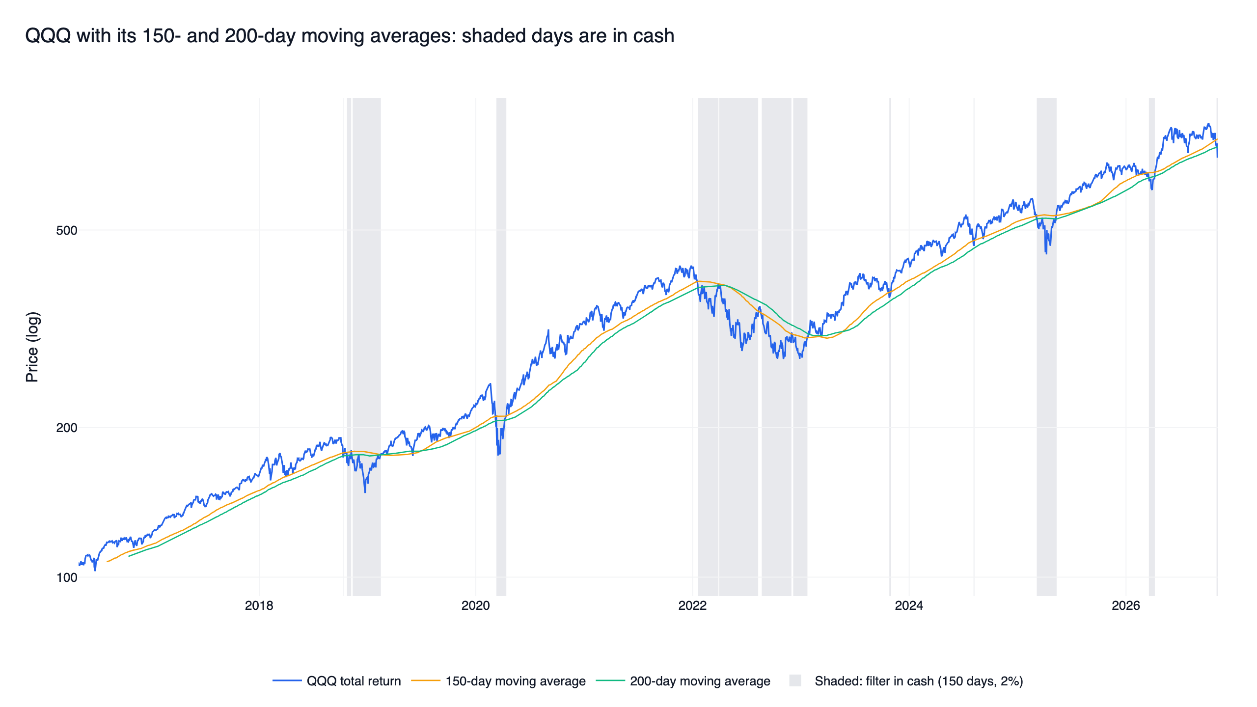
At the original setting the filter left the market 14 times from May 2016 to November 2026. The cash periods line up with late 2018, March 2020, most of 2022, spring 2025 and a short stretch in early 2026. Without a buffer the 100-day version left 57 times; the 200-day versions left 11 to 21 times.
The two strategies under the filter
Both are on our US strategy pages and passed our three robustness checks against QQQ before this test:
- Earnings-surprise breadth: counts how many of the 500 most liquid US stocks beat EPS estimates by more than 5% with a positive price reaction in the last 20 trading days. Risk-on when that count is above 1% of the universe and QQQ is above its 200-day average with positive six-month momentum.
- Free-cash-flow breadth: the share of liquid stocks with positive free cash flow, an FCF margin above 5%, debt-to-equity below 1.2 and price above their 200-day average. Risk-on above 5% with the same QQQ trend condition.
In risk-on months both hold about 25% TQQQ, 25% TECL and 50% in the strongest defensive ETF; in risk-off months only the strongest of IEF, GLD and SHY. Both rebalance monthly with an 8% stop-loss. TQQQ and TECL are 3x leveraged ETFs whose daily reset causes decay in choppy markets; the leveraged ETF timing backtest shows TQQQ held outright fell 81.7% from its peak in that window. Each script was run unchanged from its strategy page, with data through 2026-11-06; over the strategy pages' own window, the rerun matched them within 0.2 percentage points of CAGR and 0.02 of Sharpe. Charts label these as the base strategies.
The filtered version keeps everything else. Each rebalance's weights carry forward to the next rebalance, and on a day the filter switches, the strategy's actual holdings that day (excluding positions closed by the stop) are scaled by the exposure, with the rest in cash. With exposure fixed at 1, this replay matches the original strategy on every day, which is how we checked the layering.
Volatility management follows Moreira and Muir (2017) and the momentum version in Barroso and Santa-Clara (2015). At each month's last close, exposure for the next month is min(1, target / sigma), where sigma is the strategy's realised volatility over the last L days and the target is the median of sigma up to that day times m. The grid is L = 21, 63, 126 days by m = 0.8, 1.0, 1.2, with 63 days and 1.0 as the original.
How a filter had to pass
The conditions were posted before any results and not changed:
- Three robustness checks against QQQ total return: at least 7 of 9 settings with a higher daily Sharpe ratio, the original setting ahead in both halves of the window, and ahead at finlab's default US cost of zero and at 0.1% per side. For US designs it also had to beat QQQ on returns above T-bills (BIL) and without the calendar year of its largest lead.
- Better than the strategy underneath: at least 7 of 9 settings, and both halves of the original setting, with a higher Sharpe ratio on returns above T-bills than the base strategy. Cash earns nothing in the simulator, so the T-bill adjustment keeps the comparison fair.
- A different strategy: weekly returns correlated below 0.95 with the base and with every live strategy page.
Check 1 was easy here, because both base strategies already beat QQQ by a wide margin. Check 2 is the actual question.
Result: the moving average filter barely moved the numbers
Both filters passed the first group on both strategies: all 9 settings beat QQQ's Sharpe ratio, and each original setting beat it in both halves, at 0.1% per side, above T-bills and without its best year. At 0.1% per side the filtered earnings-surprise strategy still had a Sharpe ratio of 1.41 against 0.92, and without 2020, its best year against QQQ, 1.26 against 0.87. Against their own base strategies, only 1 to 4 of 9 settings came out ahead.
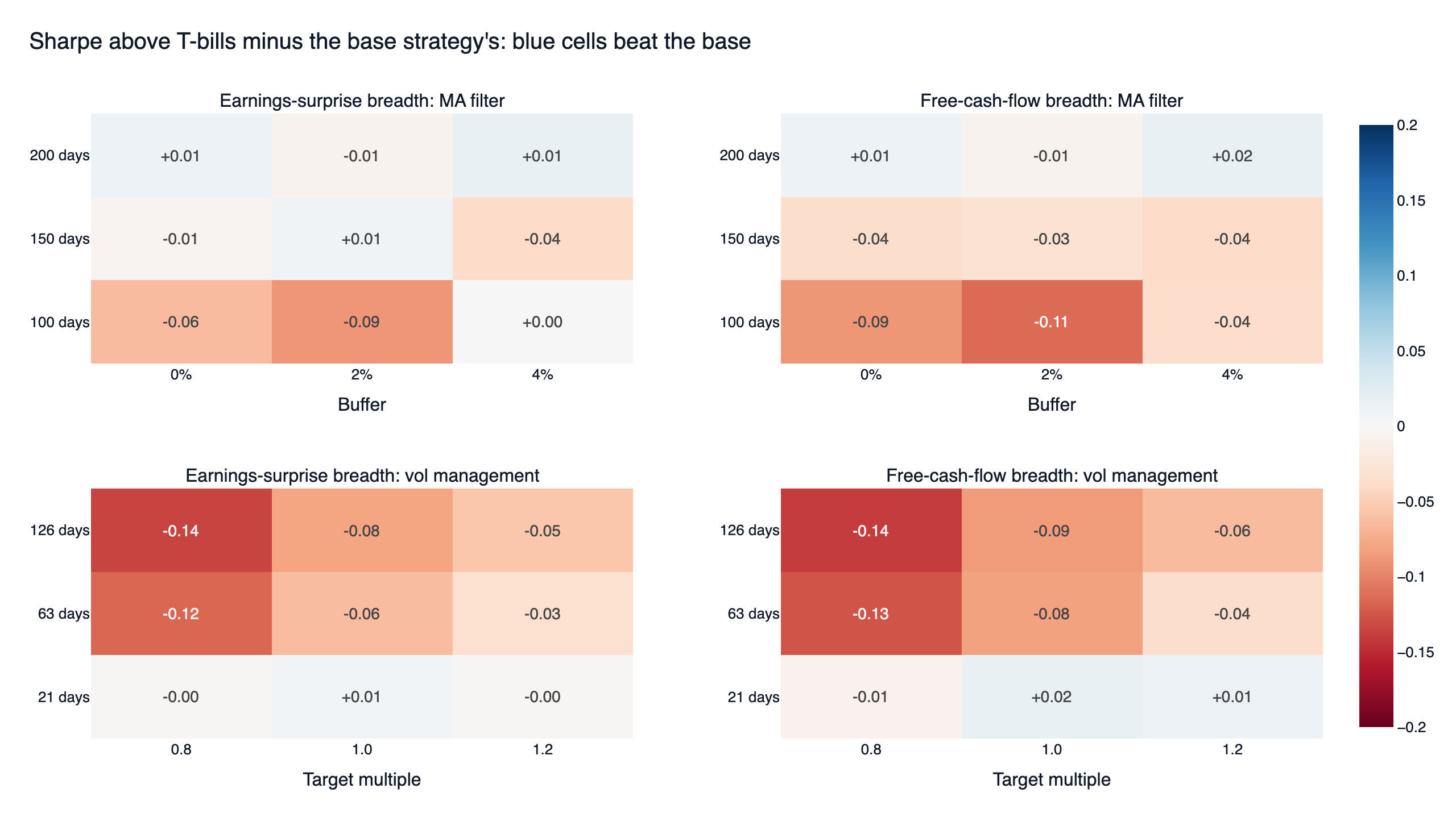
- Earnings-surprise breadth: 4 of 9 settings beat the base, by at most 0.015. The original setting added 0.009, and its second half (1.07) trailed the base (1.09).
- Free-cash-flow breadth: 2 of 9 settings beat the base, both at 200 days. The original setting lost 0.03.
- The classic 200-day rule with no buffer added 0.012 (earnings surprise) and 0.011 (free cash flow) to the Sharpe ratios above T-bills. The 100-day settings cost up to 0.11; with no buffer the 100-day average sent the strategies to cash 57 times, against 14 at the original setting.
Drawdowns improved: -21.1% to -15.3% for earnings surprise and to -18.4% for free cash flow. Return fell by about one to two points a year. That trade-off is real, but it is a matter of how much risk you want, not a better strategy, and the 0.97 weekly correlation says the filtered versions behave like the originals almost every week.
Why the filter added little
The filter can only change the days it is in cash. On those days (15.3% of the window) the two strategies were often already defensive, because their own rule needs QQQ above its 200-day average. They earned 5.5% a year (Sharpe 0.40) and 9.9% a year (Sharpe 0.74), well below their Sharpe ratios of 1.61 and 1.58 on the other days but still positive. Moving those days to cash gave up that return and that volatility in roughly equal measure.
QQQ itself tells a different story. On the days the filter was in cash, QQQ still returned 18.2% a year, with 37.1% volatility, against 21.1% and 18.5% on the other days. Below its moving average the Nasdaq 100 was not falling on average; it was swinging twice as hard, with sharp rebounds such as April 2020 and spring 2025. A filter that sits out those days removes risk, but it does not remove losses.
Volatility management cut return by a quarter
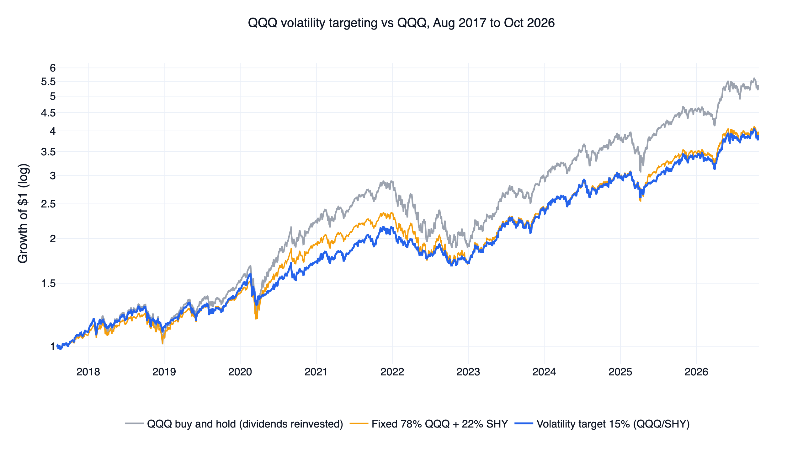
Monthly volatility management kept both strategies about 81% to 82% invested on average and cut the maximum drawdown to -17.7%. It also cut CAGR from about 31.6% to 23.9% and 31.8% to 23.4%, and the Sharpe ratio above T-bills fell from 1.35 and 1.36 to 1.29 and 1.28. Only the 21-day lookback came close to the base; the 63-day and 126-day versions lost 0.03 to 0.14. A standalone volatility target on QQQ itself, without any strategy underneath, is in the QQQ volatility targeting backtest. Cederburg et al. (2020) tested volatility management on 103 equity strategies and found that, implemented in real time, it did not reliably beat the unmanaged versions; these two strategies are consistent with that.
The same filter on 31 Taiwan strategies
We ran the identical test on the 31 Taiwan stock-selection strategies on our strategy pages, with the TAIEX total return index and its 120-day average (2% buffer) as the filter. There the result was more varied: 27 of 31 had smaller drawdowns, all 31 had lower CAGR, 17 had a higher Sharpe ratio, and 3 passed every condition (a 30-stock micro-cap strategy, a 60/40 core-satellite portfolio and an operating-margin factor strategy).
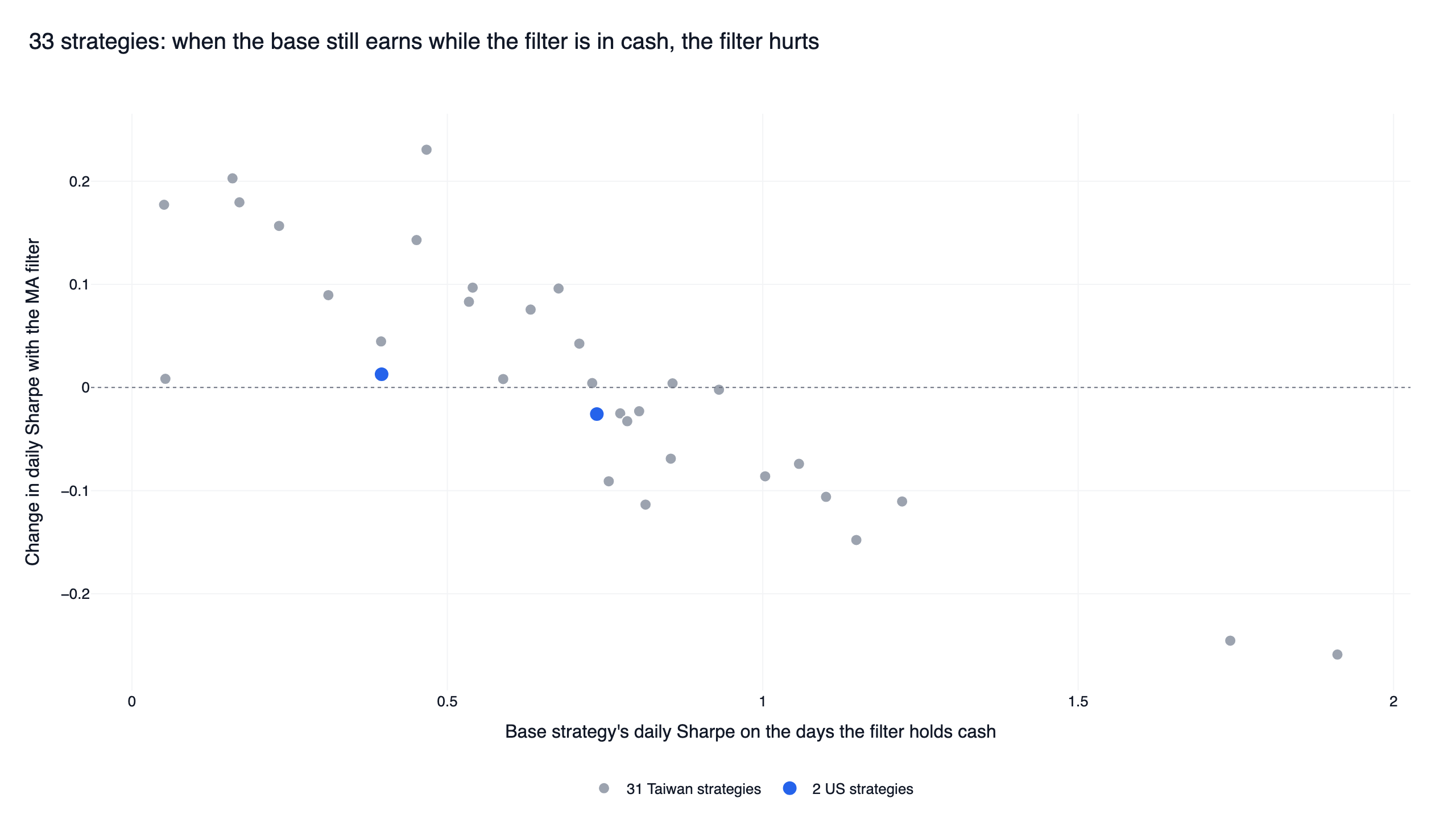
Across the 31 Taiwan strategies, the change in Sharpe had a correlation of -0.88 with how well the base strategy did on the days the filter held cash. All 9 Taiwan strategies with a Sharpe ratio below 0.5 on those days improved; all 8 above 0.9 got worse, mostly revenue-momentum strategies that kept rising while the index was weak. The two US strategies sit in the middle, at 0.40 and 0.74 on those days, and their Sharpe ratios barely moved, in line with the Taiwan pattern.
The code
The filter is a few lines in finlab. market_exposure() turns QQQ and its average into a 0/1 series, and with_market_filter() scales any finished backtest's holdings by it. This is simplified: the full research.py also handles stopped-out positions and runs every setting.
Show Code
import pandas as pd
from finlab import data
from finlab.backtest import sim

MA_DAYS = 150   # moving average length
BUFFER = 0.02   # exit only 2% below the average


def market_exposure():
    """1 = hold the strategy, 0 = cash; between the two lines keep yesterday's state."""
    data.set_market("us_fund")
    qqq = data.get("us_fund_price:adj_close")["QQQ"].dropna()
    average = qqq.rolling(MA_DAYS).mean()
    state = pd.Series(float("nan"), index=qqq.index)
    state[qqq >= average] = 1.0
    state[qqq < average * (1 - BUFFER)] = 0.0
    return state.ffill().fillna(1.0)


def with_market_filter(base_report, **sim_args):
    """Keep each rebalance's weights until the next one and scale them by the exposure."""
    days = data.get("us_fund_price:adj_close").index
    days = days[days <= base_report.creturn.index[-1]]
    weights = base_report.position[base_report.position.index < days[-1] + pd.offsets.BDay()]
    weights.index = days[days.searchsorted(weights.index, side="right") - 1]
    weights = weights[~weights.index.duplicated(keep="last")]
    days = days[days >= weights.index[0]]

    exposure = market_exposure().reindex(days, method="ffill").fillna(1.0)
    switches = exposure.index[exposure.ne(exposure.shift())][1:]
    position = weights.reindex(days, method="ffill").fillna(0.0).mul(exposure, axis=0)
    return sim(position, resample=weights.index.union(switches), upload=False, **sim_args)
Pass the base strategy's report and its own settings (for example stop_loss=0.08), and compare report.creturn with the original.
Install the FinLab skill for your AI agent
You do not need to write this yourself. Install the FinLab skill in Claude Code, Codex or Gemini CLI with one command:
Show Code
npx skills add koreal6803/finlab-ai --skill finlab -g -yThen ask your agent in plain language, for example "add a 200-day moving average filter on SPY to my strategy and compare drawdowns" or "split my backtest into days QQQ is above and below its 150-day average". The agent setup page has the details, and FinLab Studio runs the same research in a browser.
Backtest method and limits
| Item | How it was handled |
|---|---|
| Window | 2016-05-02 to 2026-11-06, the strategy pages' start; data through 2026-11-06 |
| Base strategies | The strategy pages' scripts, run unchanged; reruns within 0.2 points of CAGR and 0.02 of Sharpe |
| Signal | QQQ close with dividends reinvested against its moving average at the same close (look-ahead bias control); traded at the next day's close |
| Early months | Until QQQ had 150 or 200 days of history, the filter stayed invested |
| Volatility management | Uses only returns up to each month's last close |
| Cost | finlab sim() default US cost of zero, plus a rerun at 0.1% per side. Slippage and capacity are not estimated |
| Cash | Earns nothing in the simulator; returns above BIL are reported for that reason |
| Leverage | The strategies hold 3x ETFs in risk-on months; decay and gap risk are part of the results |
| Sample | Whole window in-sample. The halves only check stability; no out-of-sample test was run |
What this result does and does not say
Within this window, adding a QQQ moving average filter to these two strategies traded one or two points of annual return for a shallower drawdown, with no gain per unit of risk. That is specific to strategies that already follow the trend. A strategy that stays fully invested in stocks and loses money when the market breaks down could behave differently, as several Taiwan strategies did; the way to know is to split your own backtest into days above and below the average and compare.
The broader set of rules on leveraged ETFs is in the TQQQ 200-day moving average backtest. A breakout version of trend following is in the QQQ breakout trend strategy and the Turtle trading backtest.
FAQ
What is a 200-day moving average market filter?
A rule that keeps a portfolio invested only while a market index, here QQQ, is above its 200-day moving average and moves to cash when it closes below. It does not choose stocks; it switches the whole strategy on and off.
Does a 200-day moving average filter improve returns?
Not in this test. It lowered annual return by about one to two percentage points for both strategies, while cutting the maximum drawdown from -21.1% to between -15.3% and -18.4%.
Is 200 days better than 150 or 100 days?
Slightly. The 200-day settings were the only ones that beat the free-cash-flow strategy, by 0.011 to 0.016 in Sharpe above T-bills, and the 100-day settings were the worst, losing up to 0.11. None of the differences were large enough to pass.
Is the 200-day moving average a good trend following strategy on QQQ?
That is a different test from this one. TQQQ and QLD timed with a 200-day filter are covered in our leveraged ETF rules test, and the TQQQ rule failed our robustness checks there too.
What is volatility management?
Cutting exposure when a strategy's recent volatility is high and restoring it when volatility is low, so the portfolio's risk stays steadier. Here it cut CAGR by about a quarter and did not improve the Sharpe ratio.
When does a market filter help?
When the strategy underneath loses money or earns little while the market is below its average. Across 31 Taiwan strategies, the change in Sharpe had a -0.88 correlation with the base strategy's Sharpe on those days, and the two US strategies, at 0.40 and 0.74 on those days, barely changed.
Can I rerun this?
Yes. Install finlab, download research.py below and run python research.py us. It fetches each base strategy's script from our site.
Reproduce it yourself
- research.py: runs the base strategies unchanged, layers both filters at all settings and applies the three groups of checks.
python research.py usruns the two US strategies. - metrics.json: the numbers behind this article's tables and charts, including the grid, halves, cost runs, correlations and the statistics for days in and out of the market.
- data.csv: weekly equity curves of both strategies, their filtered versions and QQQ.
- metrics.json for Taiwan: the same statistics for the 31 Taiwan strategies.
For the bigger picture, start with what quantitative trading is. New research is on the FinLab blog, the team is on the about page, and the live versions of both base strategies are on their strategy pages.
Disclaimer: this article is for education only and does not constitute investment advice. Past performance does not guarantee future results, leveraged ETFs can lose most of their value, and investing involves risk. All results are in-sample, and the two halves were not validated out of sample.
Last updated: 2026-11 | Backtest window: 2016-05 to 2026-11 | Data through 2026-11-06, run 2026-11-08 | Benchmark: QQQ total return | Author: FinLab Quant Research (reviewed by a quantitative researcher)
FinLab AI
Want to build your own strategy?
Describe your stock-picking ideas in natural language. AI automatically validates, backtests, and gives you answers
Start Free