View results · Download research files
Reproduce this research
Copy the prompt to reproduce the evidence above with the article’s data, assumptions, and risk checks.
Tell your AI:
Set up FinLab and reproduce the QQQ fixed-anchor grid study
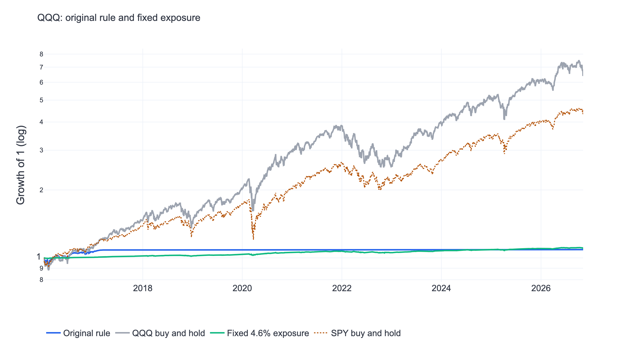
Grid trading QQQ did not pass this test. All 27 fixed-anchor settings had a lower daily Sharpe ratio than buying and holding QQQ with dividends. The original setting returned 0.78% a year, with a Sharpe of 0.31 and a maximum drawdown of -6.82%. QQQ returned 18.86% a year with a Sharpe of 0.89. Average grid exposure was only 4.64%; holding that same percentage of QQQ at a constant daily weight scored 0.89. This is a study of a failed implementation, not a strategy recommendation.
The rule sold its remaining position early in the sample. Its final positive target was on April 18, 2017. Prices then stayed above the fixed range at which it would buy again. A flat equity curve after that point represented a portfolio sitting in cash while the underlying market continued to move.
What is grid trading?
Grid trading divides prices into levels. Crossing a level down increases the position; crossing one up reduces it. A fixed-anchor grid keeps its original reference price throughout the study. It needs a return to its buying region before it can rebuild a position that it previously sold.
This differs from the trend-following rules in our US momentum research. A momentum allocation usually adds risk after strength. This grid sells into strength and buys into weakness. That is a different way to hold an asset, with different exposure to trends and reversals.
Tables scroll horizontally on smaller screens.
| Holding rule | What triggers a purchase? | What happens in an extended rise? |
|---|---|---|
| Fixed-anchor grid | Price crosses a lower grid level | Positions shrink and can reach zero |
| Constant-weight allocation | A scheduled rebalance back to target | Some shares are sold, but positive exposure remains |
| Buy and hold | The initial allocation | The original shares remain invested |
The asset here is QQQ, an ETF tracking the Nasdaq-100 according to its issuer's description. There is no stock-selection signal, short position, margin borrowing or leveraged ETF in this experiment. The US quantitative strategy comparison provides context for other holding mechanisms.
The grid trading strategy fixed before the run
We specified the rule and every neighbouring setting before inspecting returns. The centre is the first available dividend-adjusted QQQ price, and never moves. The original parameters are 5% spacing, eight cells and a 50% starting position.
| Parameter | Tested values | Original setting |
|---|---|---|
| Geometric grid spacing | 3%, 5%, 7% | 5% |
| Number of cells | 6, 8, 10 | 8 |
| Starting position | 25%, 50%, 75% | 50% |
| Anchor | First available adjusted close | Fixed throughout |
| Signal and execution | Closing signal, next-session closing execution | No same-close fills |
Take the logarithm of the ratio of today's adjusted price to the initial price, divide by the logarithm of one plus the spacing, and truncate toward zero. This gives the signed grid level. The target weight is the starting weight minus that level divided by the cell count, clipped between zero and one.
For the original setting, each level changes the target by one eighth of portfolio value. Four upward levels reduce a 50% position to zero. The upper boundary is approximately 21.6% above the initial adjusted price. This is arithmetic implied by the rule, rather than a price target fitted to the return history.
A price gap across several cells changes the next target immediately to the appropriate weight. We do not assume that each intermediate intraday limit order filled. Downward spacing is geometric, so dividing by 1.05 is slightly different from falling exactly 5%. The experiment is a closing-price allocation grid, which should not be confused with an intraday execution bot.
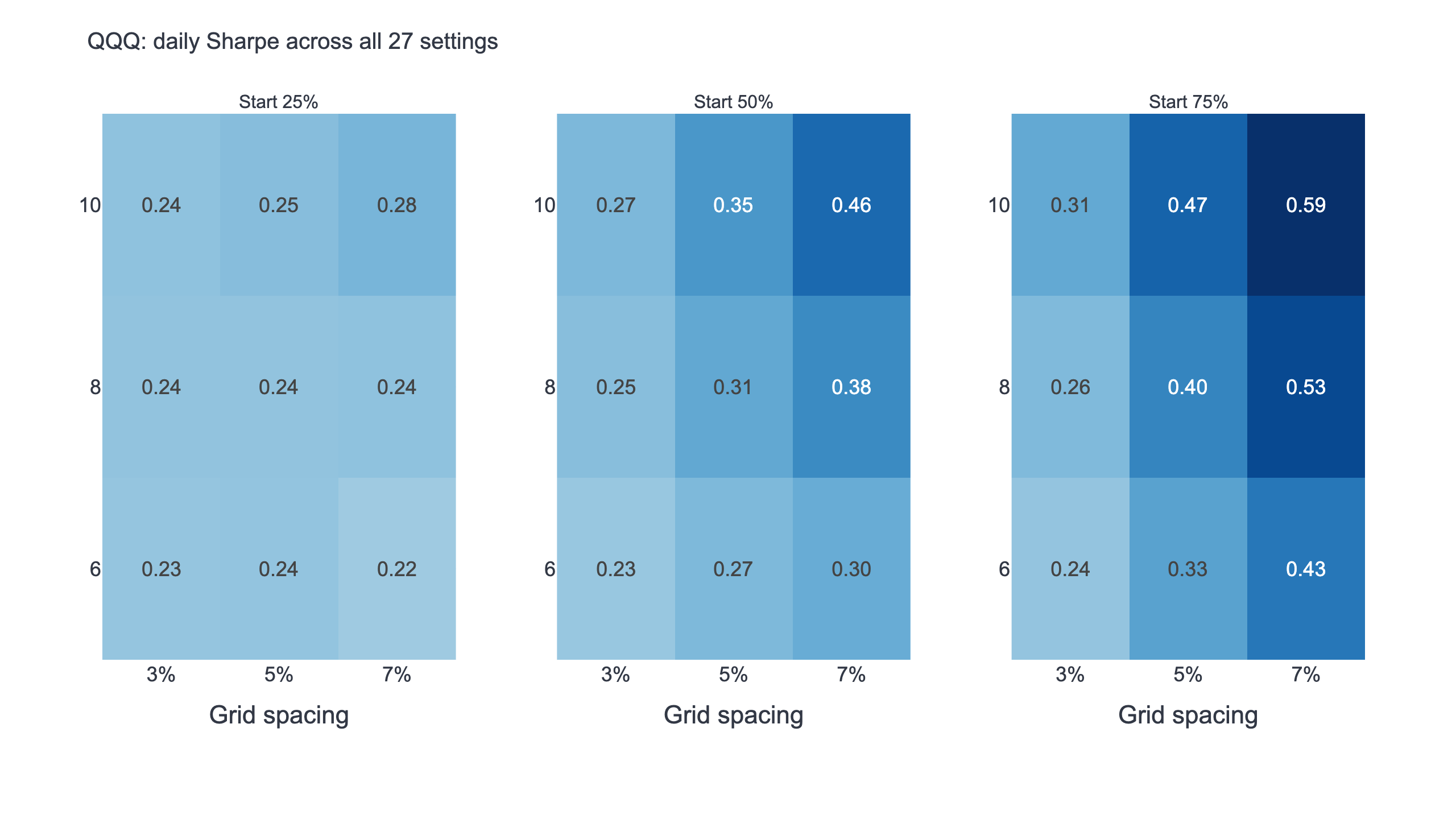
The 27 Sharpe ratios ranged from about 0.22 to 0.59, below QQQ's 0.89 over the same window. Wider ranges and larger initial holdings changed how long the grid stayed invested, but did not produce a region of robust wins. We kept the middle setting as the main result; the best historical cell did not replace it.
Comparing with the same average exposure
A small drawdown can be produced by taking very little market risk. To separate that effect from the trading rule, we measured average nominal exposure and ran a second portfolio that held that percentage of QQQ at a constant daily weight. Uninvested capital earned zero in both implementations.
The original grid averaged 4.64% exposure. This average includes the way holdings drift between trades. It does not assume that every unchanged target caused a fresh daily rebalance. The matched allocation, in contrast, was explicitly rebalanced daily.
| Metric | Original grid | Fixed 4.64% QQQ | QQQ total return | SPY total return |
|---|---|---|---|---|
| CAGR | 0.78% | 0.92% | 18.86% | 14.54% |
| Daily Sharpe | 0.31 | 0.89 | 0.89 | 0.86 |
| Maximum drawdown | -6.82% | -1.80% | -35.12% | -33.70% |
| Annualized volatility | 2.61% | 1.04% | 22.31% | 17.71% |
The constant-weight control earned more with a shallower drawdown. The grid held considerably more risk early in the period, bought during weakness, and subsequently exited. Averaging that history together with years of zero holdings creates a low exposure figure without removing the losses already incurred.
The matched weight uses the full sample and was unavailable at the beginning of the test. It is a diagnostic control, not a tradable forecast of the correct allocation. SPY is a broad-market reference; QQQ remains the required benchmark. Our Sharpe ratio guide explains why the denominator and comparison convention matter.
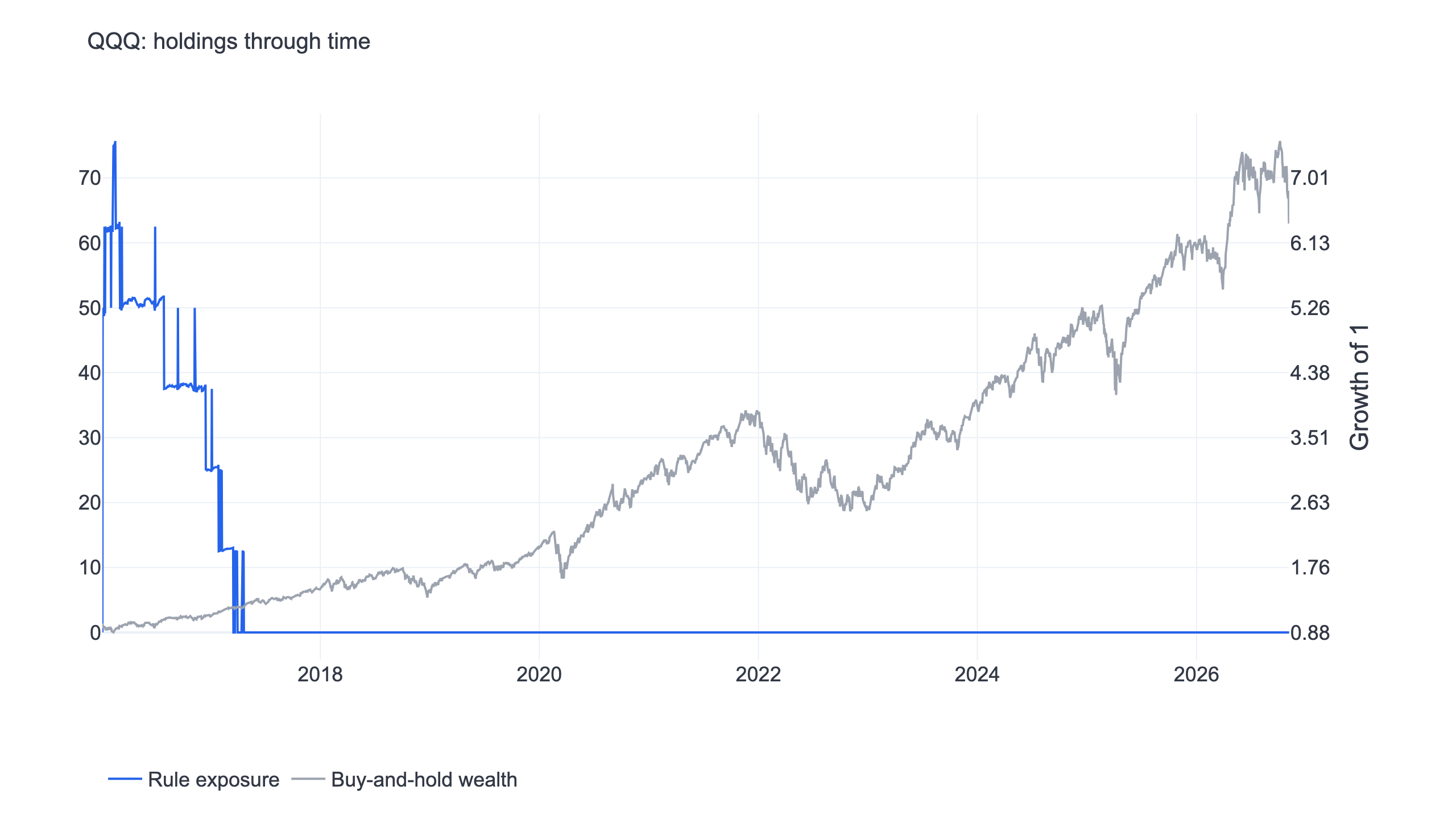
The blue line measures nominal exposure entering each return observation. The grey line uses the right axis to show QQQ total-return wealth. Once exposure reached zero, subsequent market gains contributed nothing to the grid portfolio. A flat line can therefore describe both low volatility and a large opportunity cost.
Costs and the return available on cash
FinLab's default US fund commissions and transaction taxes are zero. We also charged 0.1% on every purchase and sale. CAGR fell from 0.78% to 0.74%, and daily Sharpe fell from 0.31 to 0.30. Transaction costs made the result worse, but did not cause the original failure.
Because the grid spent so long in cash, we also subtracted each day's return on the short Treasury-bill ETF BIL before calculating Sharpe. The grid scored -0.51 against QQQ's 0.79. That comparison asks whether returns compensated for the return available on short bills. BIL was not actually held inside the simulated grid, and its return was not added to the equity curve.
The ordinary Sharpe used for the main gate subtracts no risk-free rate. Its numerator is the mean daily return; its denominator is the daily sample standard deviation, annualized by the square root of 252. A ratio above BIL answers a different question and is labelled separately. Mixing those two definitions would make the comparison misleading.
Both halves and the best-year check
Passing required at least 19 of 27 neighbouring settings to beat QQQ on daily Sharpe, the original setting to win in both halves, and a win after default trading costs. The extra cash, matched-exposure and best-year checks were also specified in advance.
| Check | Grid daily Sharpe | QQQ daily Sharpe | Result |
|---|---|---|---|
| Neighbouring settings | 0 of 27 won | About 0.89 | Failed |
| First half, Jan 2016 to Jun 2021 | 0.44 | 1.08 | Failed |
| Second half, Jun 2021 to Nov 2026 | Undefined | 0.70 | Grid held only cash |
| Cost of 0.1% per side | 0.30 | 0.89 | Failed |
| Daily returns above BIL | -0.51 | 0.79 | Failed |
| Remove best grid year, 2016 | 1.26 | 0.91 | Won this check only |
The second-half grid return and volatility were both zero. Dividing by zero gives an undefined Sharpe, rather than evidence that the grid matched a low-risk investment. We leave that entry undefined in the downloadable metrics as well.
Removing the best calendar year means removing that year's daily return observations, while retaining the original state of the strategy. We did not restart the grid at a new anchor. Without 2016, grid Sharpe rose to 1.26, but CAGR was only 0.27%. The remaining small, low-volatility gains increased the ratio. That single success did not compensate for failure on the other required checks.
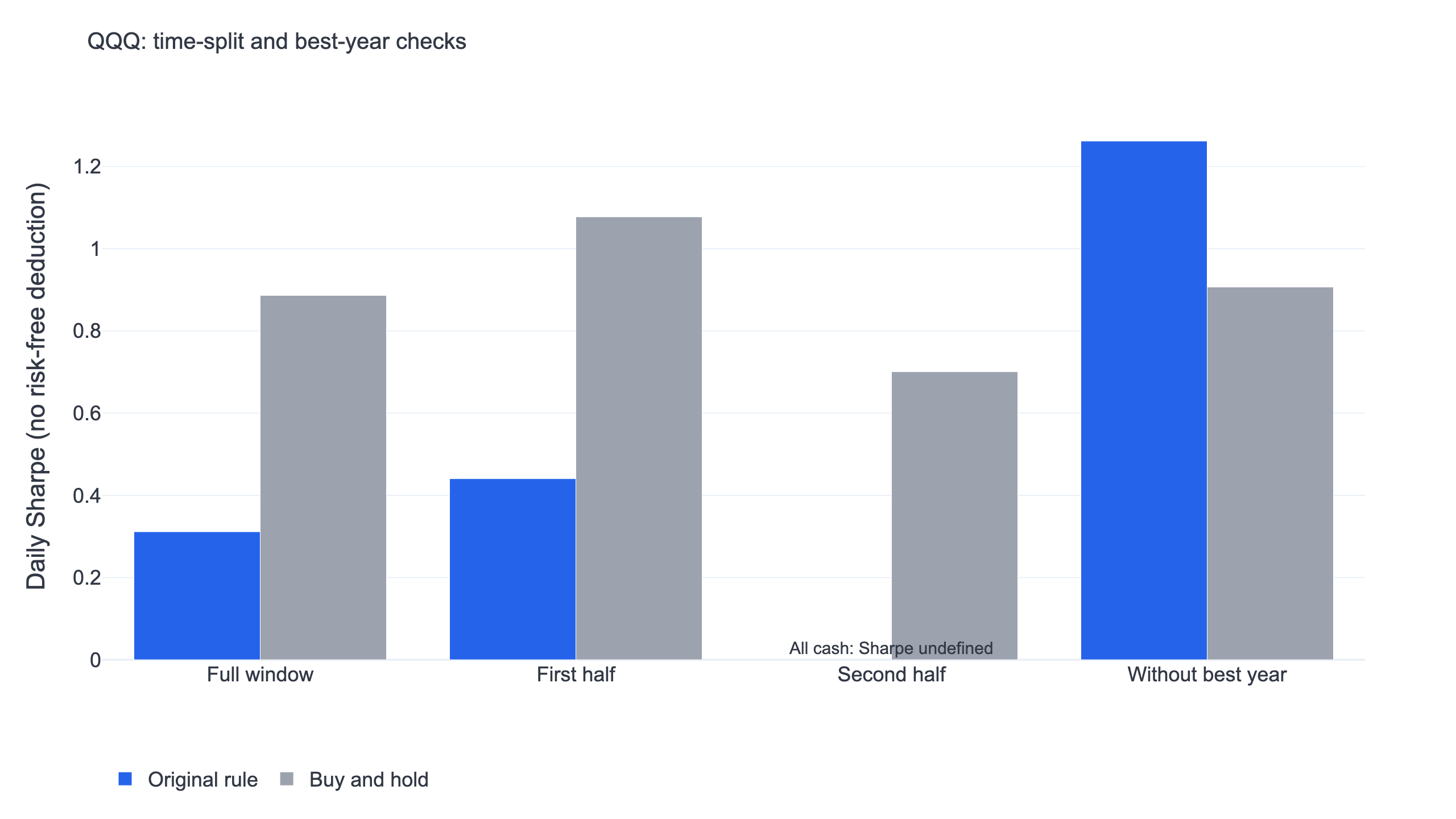
This is a useful counterexample to selecting whichever metric makes a strategy look attractive. A high ratio in a reduced sample can coexist with almost no continuing market participation. The backtesting guide discusses the importance of keeping evaluation rules fixed.
What the academic work does and does not establish
Perold and Sharpe (1988) compare dynamic allocation policies and their responses to market paths. Their framework helps explain why contrarian rebalancing and trend-following can behave differently. It does not establish that a fixed-price grid beats buy and hold.
Cover (1991) studies constant-rebalanced portfolios. A constant-weight portfolio retains an allocation, while our bounded grid can sell everything. Those mechanisms should not be treated as interchangeable evidence.
Bailey and coauthors (2015) examine backtest overfitting. Reporting all neighbouring settings and retaining the original middle cell reduces the temptation to present the most attractive historical result as a discovery. It does not turn this historical sample into a new out-of-sample test.
Data, execution and remaining limitations
Prices came from FinLab's us_fund_price:adj_close. In this run, QQQ, SPY and BIL had usable prices from January 4, 2016. The evaluation window is January 5, 2016 through November 6, 2026. We initially expected an earlier start, but did not manufacture the missing 2015 history. The run date was November 10, 2026, using FinLab 2.3.8.
The universe contains a single ETF. There is no current-constituent stock list filled backward, stock liquidity screen, delisted-stock reconstruction or financial-sector exclusion. Both the signal and benchmark use dividend-adjusted prices. A broker grid drawn on raw quoted prices needs separate treatment of distributions and splits.
The benchmark curves are calculated directly from same-window adjusted prices, without a sim() benchmark or trading costs. The strategy receives a next-session closing fill after a closing signal. Fractional weights are allowed. Minimum commissions, lot rounding, bid-ask spread, additional slippage, order rejection and market capacity were not modelled. Average monthly target-weight changes summed to about 3.1%, with a maximum of 50%; this excludes price drift itself as trading volume.
Everything is denominated in US dollars. A Taiwan-based investor would also have currency exposure. The full historical window is in-sample. The two halves are a stability check, not an untouched holdout or a live trading record. Updated source data or package versions can change subsequent reproductions.
Install the FinLab skill for your AI agent
Use the AI-assisted setup to install the FinLab skill for Claude Code, Codex or Gemini CLI. The installation command is:
Show Code
npx skills add koreal6803/finlab-ai --skill finlab -g -yThe agent guide explains the workflow. FinLab Studio is the hosted research workspace; this unsuccessful grid has no strategy-library entry or prefilled strategy launch. Give the AI the downloadable research file and ask it to reproduce the fixed-anchor grid without changing spacing, cell counts, initial weights or the cutoff date. This task is a reproduction of a failed research design, rather than a request to deploy a trading strategy.
Show Code
import numpy as np
from finlab import data
from finlab.backtest import sim

data.set_market("us_fund")
price = data.get("us_fund_price:adj_close")["QQQ"].dropna()
price = price.loc["2015-07-01":"2026-11-06"]
level = np.trunc(np.log(price / price.iloc[0]) / np.log1p(0.05))
position = (0.5 - level / 8).clip(0, 1).to_frame()
report = sim(position, upload=False, end_date="2026-11-06")
report.to_html("report_strategy.html")
The native interactive report shows the original grid. Its built-in market reference can differ from our separately calculated QQQ benchmark; use the article table and downloadable daily series for the stated comparison.
Download research files:
The shared code also produces two Taiwan-market experiments. The program is downloadable across locales; the prose, figures and report interface on this page are English. Definitions are available in the quant glossary.
Grid trading FAQ
Does a grid always make money from volatility?
No. A completed round trip can realize a gain, while the whole account still loses or misses a larger trend. Evaluate the entire portfolio, including unfilled ranges and idle cash.
Would commission-free trading fix this result?
The default run was already commission-free. Charging 0.1% per side reduced returns slightly, but the zero-cost design had already failed.
Could the anchor move upward?
Yes, but that would be another strategy. Its reset dates, retained position and parameter neighbourhood would need to be defined and tested separately. We did not add resets after seeing this failure.
Could idle cash earn Treasury-bill returns?
That is a possible alternative allocation. This experiment kept cash at zero return and used BIL only as a comparison. It did not simulate a QQQ-plus-BIL grid portfolio.
Why did removing the best year improve Sharpe?
The remaining returns had very little volatility. Their ratio rose even though CAGR was only 0.27%. This illustrates why passing one supplementary check cannot replace all the required tests.
Does this cover leveraged ETF or intraday grids?
No. There is no TQQQ, derivatives, margin or intraday execution. Leveraged ETFs reset daily and have path-dependent returns, so QQQ results cannot simply be multiplied by a leverage factor. For a different execution mechanism, see the ETF rotation study.
Investing involves risk. Past performance does not indicate future results. This material is for research and education and does not constitute investment advice.
Last updated: 2026-11 | Backtest window: 2016-01-05 to 2026-11-06 | Author: FinLab Quant Research. The team studies Taiwan and US strategies using FinLab data and Python, retaining research definitions and reproduction code.
FinLab AI
Want to build your own strategy?
Describe your stock-picking ideas in natural language. AI automatically validates, backtests, and gives you answers
Start Free