Run this strategy
Copy the prompt to reproduce the evidence above with the article’s data, assumptions, and risk checks.
Tell your AI:
Set up FinLab and reproduce the factor ETF comparison. Please read: https://finlab.finance/en/setup?relatedUrl=/en/blog/factor-etf-qual-usmv-backtest
QUAL returned 13.9% a year and USMV 10.8%, against QQQ's 19.4% and SPY's 14.9%, from January 2016 to October 2026. USMV's annual volatility was lower, but its maximum drawdown still reached -33.1%. Rotating between MTUM, QUAL, USMV and VLUE came close to QQQ on full-period daily Sharpe, 0.88 against 0.89, yet only 3/9 settings won and the original lost the first half. This study reports a failed rotation design, with the fund comparisons as context; it does not propose a validated trading strategy.
A factor ETF packages a repeatable preference for stocks with a characteristic such as quality, value, momentum or low volatility. That characteristic can change the path of returns without increasing the final return. The question here is concrete: what did owning each fund deliver, and did switching between the factor funds improve risk-adjusted performance over simply holding QQQ?
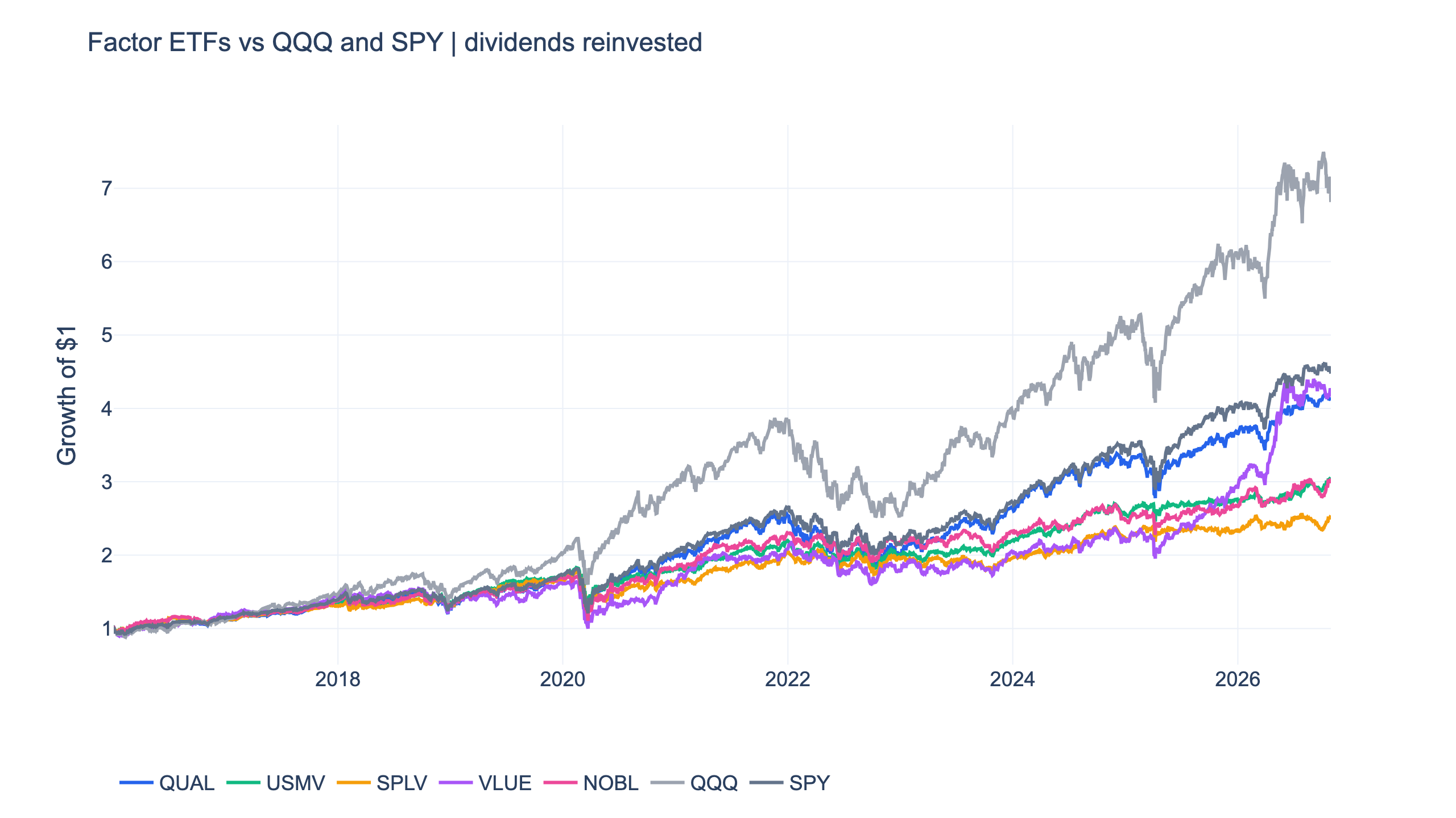
QUAL, USMV and the other factor ETFs on one window
| ETF | Total return | CAGR | Daily Sharpe | Max drawdown | First / second half Sharpe |
|---|---|---|---|---|---|
| QUAL | 310.8% | 13.9% | 0.83 | -34.1% | 0.89 / 0.76 |
| USMV | 202.6% | 10.8% | 0.79 | -33.1% | 0.85 / 0.74 |
| SPLV | 154.0% | 9.0% | 0.65 | -36.3% | 0.71 / 0.58 |
| VLUE | 318.4% | 14.1% | 0.77 | -39.5% | 0.71 / 0.84 |
| NOBL | 204.3% | 10.8% | 0.71 | -35.4% | 0.86 / 0.53 |
| QQQ | 581.2% | 19.4% | 0.91 | -35.1% | 1.08 / 0.74 |
| SPY | 347.3% | 14.9% | 0.87 | -33.7% | 0.93 / 0.82 |
These are adjusted-price buy-and-hold returns over 2016-01-04 to 2026-10-30. Dividends are reinvested, and each fund is compared with the same QQQ and SPY dates. The table separates total return, compounding and risk: a lower-volatility fund may feel easier to hold while still accumulating much less capital. None of the five factor funds exceeded QQQ's full-period daily Sharpe on this window. QUAL was closest at 0.83, followed by USMV at 0.79.
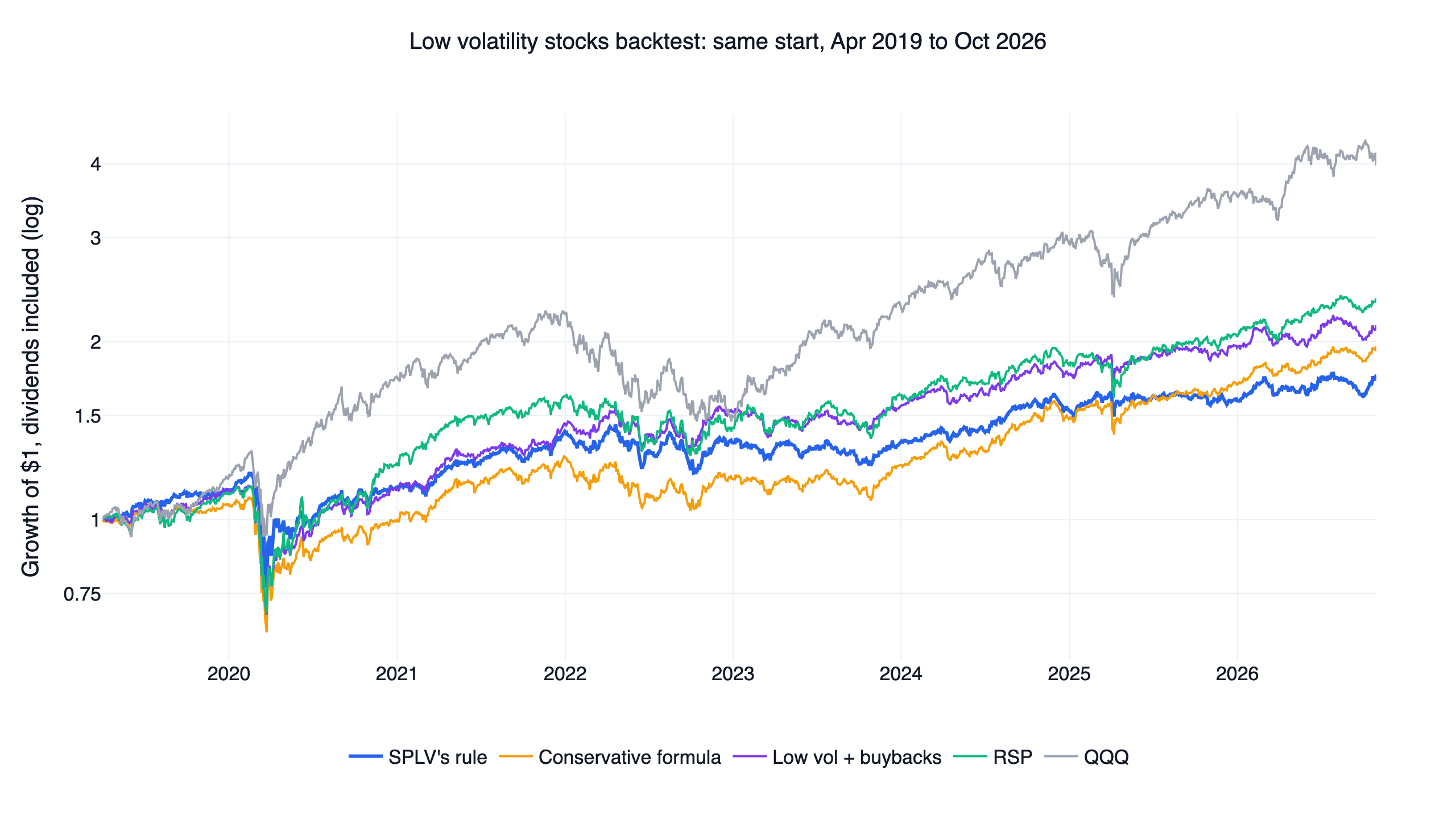
USMV's 14.2% annual volatility was below QQQ's 22.2%, and SPLV's was 15.1%. Those are substantial differences in ordinary day-to-day variation. But USMV's -33.1% drawdown was only about two percentage points shallower than QQQ's -35.1%; SPLV fell -36.3%, deeper than QQQ. A minimum-volatility or low-volatility label describes portfolio construction, without promising a loss ceiling during a market-wide shock.
Quality factor ETF: what QUAL selects
MSCI's sector-neutral quality index description uses return on equity, leverage and earnings variability. That combination distinguishes QUAL from a pure profitability portfolio and from a simple list of stable companies. Sector-relative selection also matters: the objective is to select quality within sectors, rather than to eliminate every economically sensitive industry.
Novy-Marx (2013) provides evidence for gross profitability as a return predictor. It motivates examining quality, but gross profit divided by assets is not the same signal as QUAL's three-part index score. Our test uses the ETF's actual adjusted share price, including the issuer's implementation and expenses, rather than claiming to reconstruct that academic portfolio.
QUAL's CAGR of 13.9% was about one point below SPY's and more than five points below QQQ's. Its drawdown, -34.1%, was close to both broad-market funds. The first-half Sharpe was 0.89 against QQQ's 1.08, then the second half edged QQQ 0.76 to 0.74. This is an example of changing relative performance over time, rather than evidence that the factor is permanently inferior or a reason to choose it using only the later half.
USMV vs SPLV: minimum volatility is a different rule
SPLV uses a direct low-realised-volatility selection from the S&P 500, while USMV uses MSCI's portfolio minimum-volatility approach, accounting for the way stocks move together under constraints. Invesco's SPLV description identifies the 100 least-volatile S&P 500 stocks and quarterly reconstitution. MSCI's methodology update moved its standard minimum-volatility reviews to quarterly from August 2025. That change should not be confused with an ETF's dividend-payment frequency.
Ang, Hodrick, Xing and Zhang (2006) found low subsequent returns for high-idiosyncratic-volatility stocks. The study is relevant to the low-volatility question, but neither ETF is a direct reproduction of that regression-sorted portfolio. Lower realised portfolio volatility, a stock-selection premium and protection in the worst drawdown are distinct claims. Our figures support the first for both USMV and SPLV; they do not support treating either as a strong crash hedge.
An investor also has to distinguish low volatility from low risk in every sense. A portfolio can have smooth ordinary returns while retaining equity-market exposure, sector tilts and interest-rate sensitivity. This experiment does not estimate future correlations or guarantee the largest historical drawdown will be the largest possible loss.
VLUE and NOBL: value and dividend growth are separate exposures
MSCI's enhanced value description uses price to book, forward earnings and enterprise value to operating cash flow. ProShares describes NOBL as exposure to S&P 500 companies with at least 25 consecutive years of dividend growth. Paying a high current yield is a different criterion from raising dividends repeatedly; NOBL is therefore not interchangeable with a highest-yield screen.
VLUE returned 14.1% a year with the deepest drawdown here, -39.5%, and improved from a 0.71 Sharpe in the first half to 0.84 in the second. NOBL returned 10.8% with a -35.4% drawdown and went the other way, from 0.86 to 0.53. We use their market-price histories, so no attempt is made to infer a historical 25-year dividend streak from FinLab's shorter corporate-action history. The fund itself implements that selection rule.
The original four-factor rotation, now with full history
An earlier covered call, dividend and factor study used SPMO, SPHQ, SPLV and RPV because the original four funds lacked sufficient price history. That experiment remains a test of those substitute funds. Here we rerun the intended MTUM/QUAL/USMV/VLUE design after the data history was restored, preserving the original L=9/12/15 months and k=1/2/3 settings, with L=12 and k=2 as the original.
At each month end we rank the four ETFs by trailing adjusted-price return and hold the top k in equal weight. A month is 21 trading days, matching the earlier protocol. No trend filter, stop-loss, leverage or short position is added. All nine settings start at the first month end with a full 15-month lookback, 2017-04-28, so a shorter lookback does not get a more favourable sample.
Asness, Moskowitz and Pedersen (2013) motivates examining value and momentum together across assets. It does not establish that a momentum ranking across four US factor ETFs must beat QQQ. That narrower implementation is precisely what the following test checks.
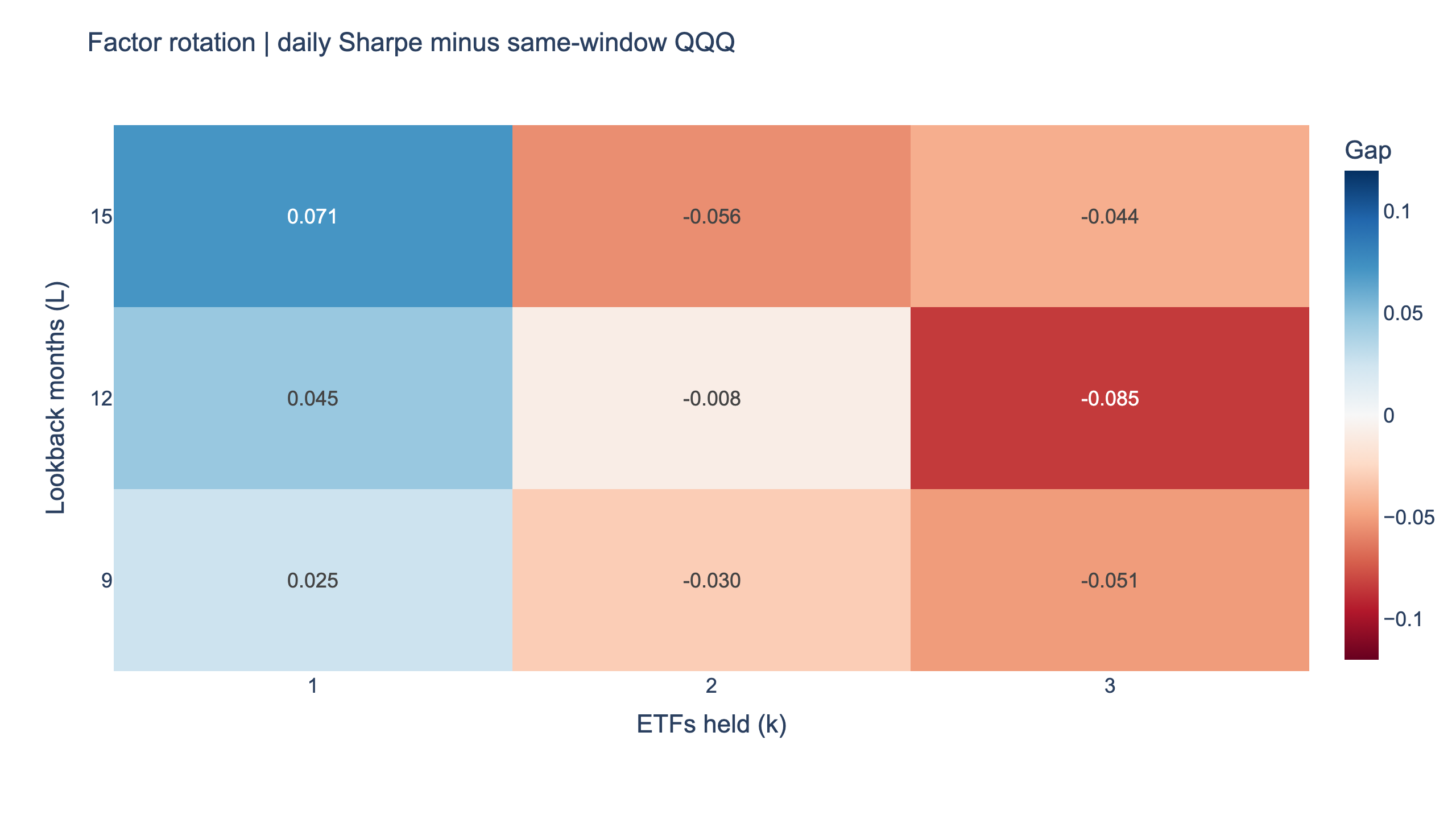
| Design | Daily Sharpe | Same-window QQQ | CAGR | Max drawdown | Winning settings | Sharpe after 0.1% per side |
|---|---|---|---|---|---|---|
| D | 0.88 | 0.89 | 16.1% | -33.6% | 3/9 | 0.86 |
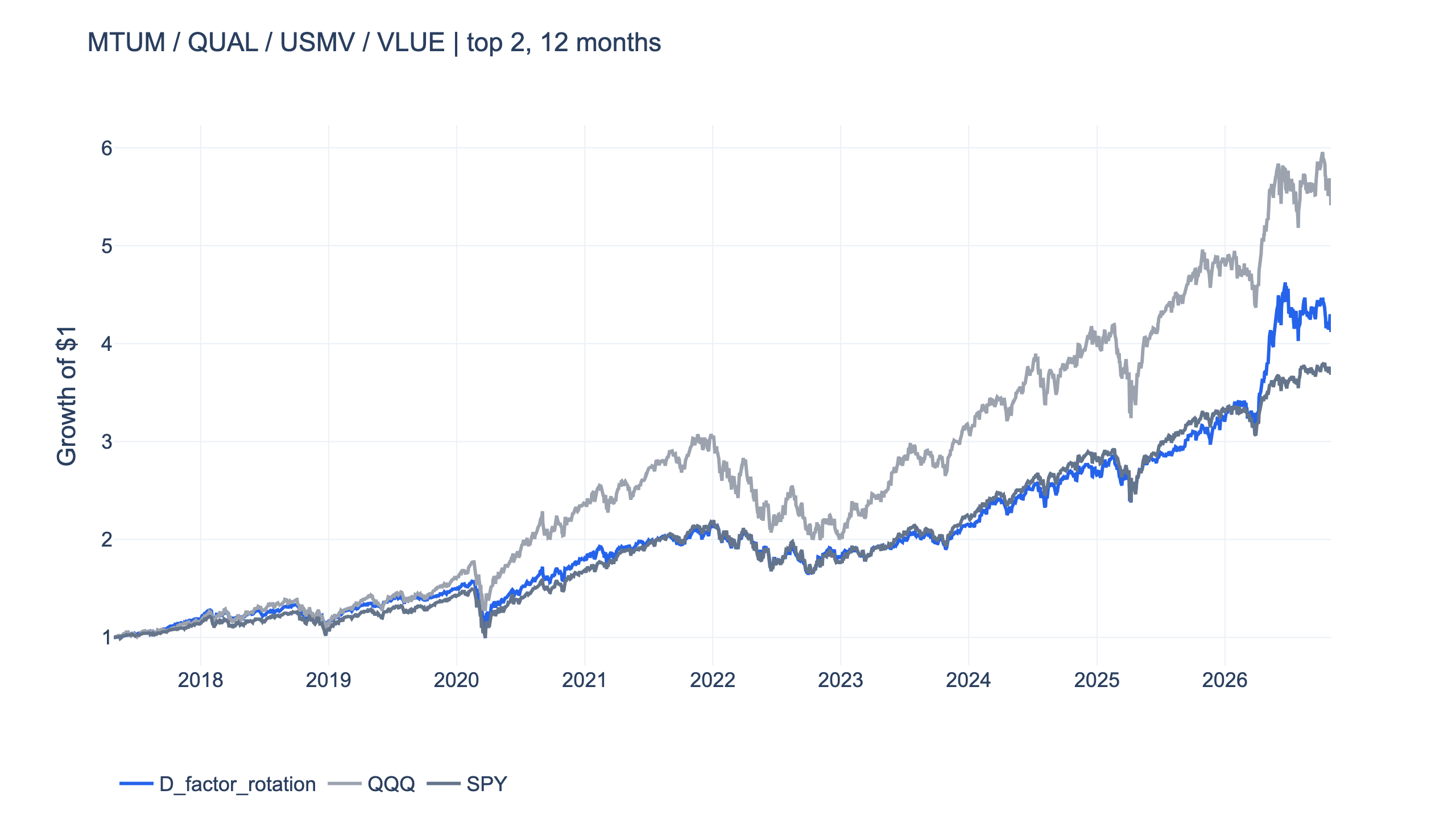
The original returned 16.1% a year against QQQ's 19.4% over those dates, with a -33.6% drawdown against -35.1%. The small Sharpe gap should be read before rounding: the values are approximately 0.8781 and 0.8865. Rounding both to one decimal would make them look identical, but it would not make the strategy win.
All three robustness checks
| Check | Observed result | Requirement | Verdict |
|---|---|---|---|
| Neighbouring parameters | 3 of 9 win | At least 7 of 9 | Fails |
| First half | 0.83 vs QQQ 1.00 | Higher daily Sharpe | Fails |
| Second half | 0.93 vs QQQ 0.77 | Higher daily Sharpe | Passes this half |
| Cost stress | 0.86 vs QQQ 0.89 | Still higher at 0.1% per side | Fails |
The chronological split is 2022-01-26. Both halves retain their own same-date QQQ returns. These halves are a stability diagnostic on an already observed sample, not a claim that the second half was an untouched holdout. The rules and neighbours were recorded before the present run, but the fund universe and research question were chosen with knowledge of the broader historical market.
A fixed-average-weight comparison helps isolate switching. The original rotation averaged about 32.5% MTUM, 29.4% QUAL, 18.0% USMV and 20.2% VLUE across monthly decisions, excluding the last observation with no subsequent holding period. Rebalancing those weights monthly gave a 0.80 daily Sharpe, below the rotation's 0.88. The rotation improved on that control while still falling short of QQQ. Since the weights are computed from the completed sample, this control is an attribution exercise, not an alternative strategy selected in advance.
After deducting daily BIL returns, the original scored 0.75 against QQQ's 0.78. Thus the result does not change when Treasury-bill returns are treated as the risk-free alternative. The three neighbouring settings that won are all top-one versions; that concentration of successes does not satisfy the preregistered broad-parameter requirement.
The separate funds do not win the same periods
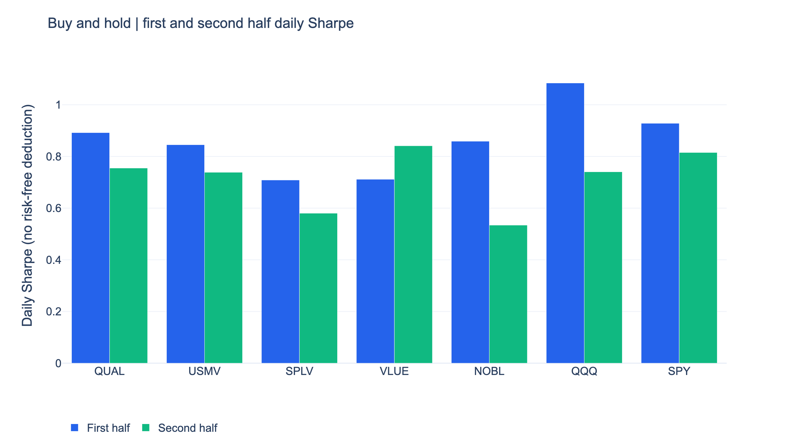
QQQ's first/second-half Sharpe was 1.08/0.74 over the full fund window. QUAL and VLUE beat it only in the second half; USMV was very close in that half and still slightly lower before rounding. SPLV and NOBL lost both halves. SPY also won only the second. Those changes are why a factor label or an appealing recent chart is insufficient for declaring an ETF superior. The figure includes every row of the holding table and uses one shared split date.
Reproduce the four-factor rule
Show Code
import finlab
from finlab import data
from finlab.backtest import sim
from finlab.markets.us import USFundMarket

finlab.login()
data.set_market("us_fund")
data.truncate_end = "2026-10-30"
calendar = data.get("us_price:adj_close").index
price = data.get("us_fund_price:adj_close").reindex(calendar).ffill()
etfs = ["MTUM", "QUAL", "USMV", "VLUE"]
score = price[etfs] / price[etfs].shift(252) - 1
selected = score.rank(axis=1, ascending=False, method="first") <= 2
weights = selected.astype(float) / 2
class QQQMarket(USFundMarket):
    @staticmethod
    def get_benchmark():
        return price["QQQ"]

report = sim(weights.loc["2017-04-28":], resample="M", market=QQQMarket(), upload=False)
report.to_html("factor_rotation.html")
The full research.py below aligns to the stock-market calendar, carries isolated missing prices forward after a fund's first quote, and includes the zero-return interval before the first simulated fill. It runs all nine factor settings and three related momentum designs, writes HTML reports and saves daily equity. That shared engine makes the two articles reproducible without changing the selection universe silently.
Install the FinLab skill for your AI agent
Start with the AI-assisted setup. The FinLab skill works with Claude Code, Codex and Gemini CLI; the agent setup guide explains the choices. Install it with:
Show Code
npx skills add koreal6803/finlab-ai --skill finlab -g -yThen ask your agent to reproduce this study using the downloaded research.py and the fixed end date. You can inspect the same code in the browser at FinLab Studio. Reproduction comes before experimenting with a new rule: confirm the original output, save a copy, and label any later change as a new experiment. Changing the rule after seeing these figures would remove the meaning of the original nine-setting check.
The interactive report uses QQQ as its market benchmark. Its display starts at the first simulated fill; the tables retain the preceding signal-date cash observation to include initial trading costs. That one-session difference can slightly change the displayed benchmark CAGR.
Method and limits
| Item | Choice |
|---|---|
| Data snapshot | Through 2026-10-30; rerun 2026-11-02 Taipei; finlab 2.3.0, pandas 3.1.0 |
| Benchmarks | QQQ primary, SPY context; direct adjusted-price buy and hold, no simulated benchmark costs |
| Execution | Month-end signals, next-close fills; up to k funds, equal weight, no leverage or shorts |
| Costs | US sim defaults are zero commission/tax; original rerun at 0.1% per buy and sell; no separate dividend/capital-gains tax model |
| Turnover | Mean target-weight turnover 10.5% per monthly decision, maximum 50.0%; half absolute weight changes, initial allocation and price drift excluded |
| Capacity | No volume filter or capacity estimate; actual spreads and price impact are not measured; fee stress is a scenario rather than a fill model |
| Selection | Named surviving ETFs chosen for this question; not every fund ever launched and not a reconstructed stock-factor universe |
| Timing and sample | Historical ETF prices rather than today's stock holdings; all in sample, no independent out-of-sample test |
FAQ
Is QUAL a substitute for QQQ?
It is a different allocation. Over this window it had lower CAGR and lower daily Sharpe, and a similar maximum drawdown. Its quality screen does not make it a Nasdaq 100 portfolio.
Which performed better, USMV or SPLV?
USMV had higher CAGR and Sharpe and a shallower drawdown here. Their selection methods differ, and this one window cannot promise the same ordering in the future.
Is a minimum volatility ETF safe in a crash?
It remains an equity ETF. USMV's historical maximum loss from a peak was about 33%, despite much lower daily volatility than QQQ.
Is NOBL a high-dividend ETF?
Its defining condition is a long history of dividend increases, rather than the highest current yield. Its actual return still depends on share-price changes and the stocks selected by that rule.
Did restoring historical prices validate factor rotation?
No. It made the intended experiment possible. The original then failed the parameter, first-half and cost checks. Data completeness and a positive strategy result are separate questions.
Why not change k to one after seeing the winners?
That would select a setting after observing the sample. The registered original was two funds and the passing rule required seven of nine neighbours. A new top-one design would need its own preregistration and future evidence.
Download the shared research
- strategy.py: the same complete research program for this article.
- research.py: the full four-design engine; running it writes the data beside the script.
- data.csv and metrics.json: the shared snapshot, including the factor holding table, nine rotation results, halves and controls.
- Original rotation report and fixed-weight baseline.
More comparisons are in the US quant trading strategies overview, the US factor investing overview, the sector rotation study, the lazy portfolio test, and the covered call and dividend study. The definitions of look-ahead bias and turnover explain two common reasons for overstating a trading rule's return. For six momentum funds and trend filters, use the companion SPMO, MTUM and momentum ETF study.
Last updated: 2026-11 | Data through: 2026-10-30 | Rerun: 2026-11-02 (Taipei) | Author: FinLab Quant Research. We publish reproducible rules, sensitivity tests and the underlying data so readers can inspect the research method.
Past performance does not represent future results. All results are in-sample backtests. Named ETFs describe research instruments and are not recommendations. This educational content does not constitute investment advice.
FinLab AI
Want to build your own strategy?
Describe your stock-picking ideas in natural language. AI automatically validates, backtests, and gives you answers
Start Free