Run this strategy
Copy the prompt to reproduce the evidence above with the article’s data, assumptions, and risk checks.
Tell your AI:
Set up FinLab and split TQQQ's yearly return into volatility decay and costs. Please read: https://finlab.finance/en/setup?relatedUrl=/en/blog/leveraged-etf-decay
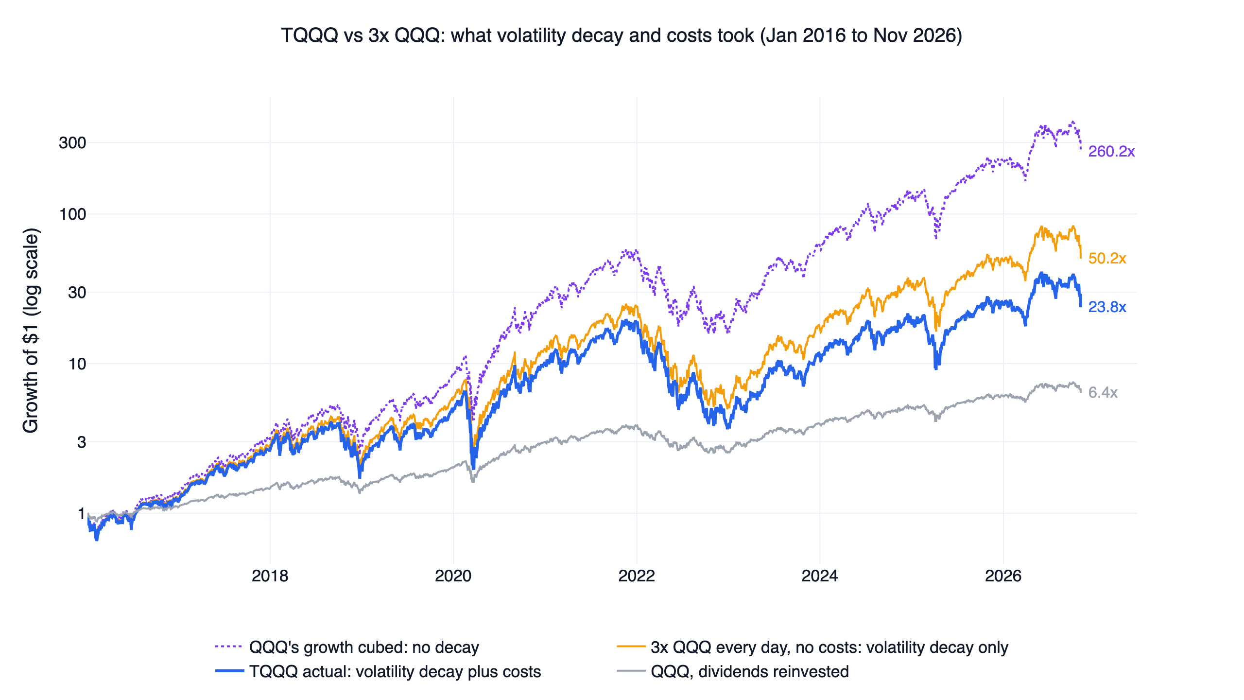
Leveraged ETF decay has two sources, and each can be measured on its own. We split the returns of 14 US leveraged ETFs from January 2016 to November 2026 with finlab. TQQQ's log return trailed three times QQQ's by 22.1 points a year: 15.2 points came from the daily reset (volatility decay) and 6.9 from fees and financing. In annual returns, QQQ with dividends made 18.7% a year. A fund that tripled QQQ's log return would have made 67.2%. Charging only the volatility decay leaves 43.6%, and TQQQ actually made 34.0%. The volatility decay follows the textbook formula closely: across 602 fund-quarters, the measured value and the formula differ by 0.13 points on average. The cost term follows short-term interest rates. In 2023 and 2024, when Treasury bills paid about 5%, TQQQ's cost term reached 12 to 13 points a year.
The decay is also concentrated. Days that opened with QQQ's 20-day volatility above 25% were 22.5% of trading days and carried 52.7% of TQQQ's volatility decay. A common response is to hold the unleveraged ETF whenever volatility is high. We tested that switch on TQQQ, QLD, UPRO and SOXL, and none passed. The TQQQ version had a daily Sharpe ratio of 0.97 against 0.90 for QQQ with dividends and held up in both halves, after costs and without its best year, but only 4 of its 9 neighbouring settings beat QQQ. The QLD version came closest, with 6 of 9.
Leveraged ETF decay: key numbers
| Fund | Leverage and underlying | Underlying volatility | Volatility term per year | Cost term per year | Total per year | Fund CAGR | Underlying CAGR |
|---|---|---|---|---|---|---|---|
| SSO | 2x SPY | 17.7% | -3.2 | -3.9 | -7.0 | 22.2% | 14.5% |
| QLD | 2x QQQ | 22.3% | -5.0 | -3.8 | -8.8 | 29.0% | 18.7% |
| TMF | 3x TLT | 14.6% | -6.4 | -6.4 | -12.9 | -14.1% | -0.8% |
| CURE | 3x XLV | 16.7% | -8.5 | -7.0 | -15.5 | 17.5% | 11.1% |
| UDOW | 3x DIA | 17.3% | -9.3 | -6.8 | -16.1 | 22.5% | 12.9% |
| UPRO | 3x SPY | 17.7% | -9.6 | -7.0 | -16.6 | 27.2% | 14.5% |
| EDC | 3x EEM | 21.0% | -13.7 | -7.2 | -20.9 | 2.6% | 8.1% |
| TQQQ | 3x QQQ | 22.3% | -15.2 | -6.9 | -22.1 | 34.0% | 18.7% |
| SQQQ | -3x QQQ | 22.3% | -30.1 | +7.4 | -22.7 | -52.4% | 18.7% |
| TNA | 3x IWM | 22.7% | -16.0 | -7.1 | -23.1 | 5.9% | 10.1% |
| TECL | 3x XLK | 24.7% | -18.6 | -7.2 | -25.8 | 40.4% | 22.0% |
| YINN | 3x FXI | 27.3% | -22.2 | -7.2 | -29.4 | -19.5% | 2.6% |
| LABU | 3x XBI | 32.6% | -32.3 | -8.0 | -40.3 | -16.6% | 7.7% |
| SOXL | 3x SOXX | 34.5% | -36.7 | -8.0 | -44.7 | 35.2% | 28.3% |
The window is 2016-01-04 to 2026-11-05, 10.8 years, on dividend-adjusted prices. The three middle columns are log points per year: the fund's log return equals the leverage times the underlying's log return, plus the volatility term, plus the cost term. Log returns add, so the two terms sum to the total, give or take 0.1 from rounding. Rows are sorted by the total, and the funds with the most volatile underlyings sit at the bottom.
Why leveraged ETFs decay: two sources
The first source is the daily reset. A leveraged ETF promises a multiple of one day's return and resets its exposure to 2x or 3x at every close. Take an index that rises 10% one day and falls 10% the next. It ends at 1.10 × 0.90 = 0.99, down 1%. A daily 3x fund ends at 1.30 × 0.70 = 0.91, down 9%, which is 6 points worse than three times -1%. Cheng and Madhavan (2009) showed that this daily rebalancing makes long-run returns path dependent. Avellaneda and Zhang (2010) wrote it as a formula. A leveraged ETF's log return is about k times the underlying's log return, minus k(k−1)/2 times the sum of squared daily returns over the period, where k is the leverage. In the example, 3 × 2 ÷ 2 × (0.1² + 0.1²) = 0.06, in line with the 6 points (the exact log gap is 0.064). This term goes by three names, volatility decay, volatility drag and beta slippage. All three mean the same thing.
The second source is fees and financing. A 3x fund holds 1 of assets, and gets the extra $2 through swaps or futures. That costs about twice the short-term interest rate plus a spread, on top of the management fee. Each extra point of short-term rates should therefore cost a 3x fund about 2 points a year, and a 2x fund about 1 point. Inverse funds work the other way. A -3x fund earns interest on its assets and on the cash from its short exposure, so higher rates help it.
In this article the cost term is everything left after the volatility term. Besides fees and financing it includes swap spreads, how the fund handles the index's dividends, and the gap between the closing price and the fund's net asset value.
How the split works: one QQQ path, three curves
The chart at the top turns one QQQ path into three curves. The dashed line at the top is QQQ's return cubed: every day's log return is exactly three times QQQ's, with no decay. Over ten years, 260.2. The middle line is a daily 3x QQQ with no costs, reset every day like a real leveraged ETF but charged nothing. 50.2, and the gap from the top line is the volatility term. The solid line is TQQQ with dividends, at 6.40 over the same dates.
Why use QQQ cubed rather than the familiar "3 × QQQ's return"? Three times a simple return already understates a decay-free fund. If QQQ gains R in a year, the cube is (1 + R)³ − 1, which exceeds 3R by R²(3 + R). R cannot fall below -100%, so that gap is never negative. In 2023 QQQ rose 54.9%: three times that is 164.6%, while the cube is 271.3%. A year when TQQQ beats 3x QQQ can still be a year with decay. The yearly table below shows TQQQ up 198.3% in 2023 while the two terms still took 21.9 log points.
Every split is computed separately for each calendar year and each quarter. The fund's and the underlying's returns come from the prices at the start and end of the period. The no-cost return chains the underlying's daily returns times k across every day in between.
Checking the prices first
The split only works if each fund's daily return really is close to k times its underlying's. We compared every fund's daily returns with k times the underlying's. All 14 funds in the main table have a correlation of at least 0.9975. Their realized multiples, the regression slopes, run from 2.94 to 2.99 for the 3x funds, and SQQQ's is -2.96. TQQQ, for example, has a correlation of 0.9989 and a slope of 2.96. On only 1 of 2,726 trading days was it more than 2 points away from three times QQQ.
One fund was left out. TYD, a 3x fund on 7-10 year Treasuries, has a correlation of only 0.9093 with three times IEF and was more than 2 points off on 35 days. It trades thinly and its closing price often strays from its net asset value.
Result 1: the volatility term follows the formula
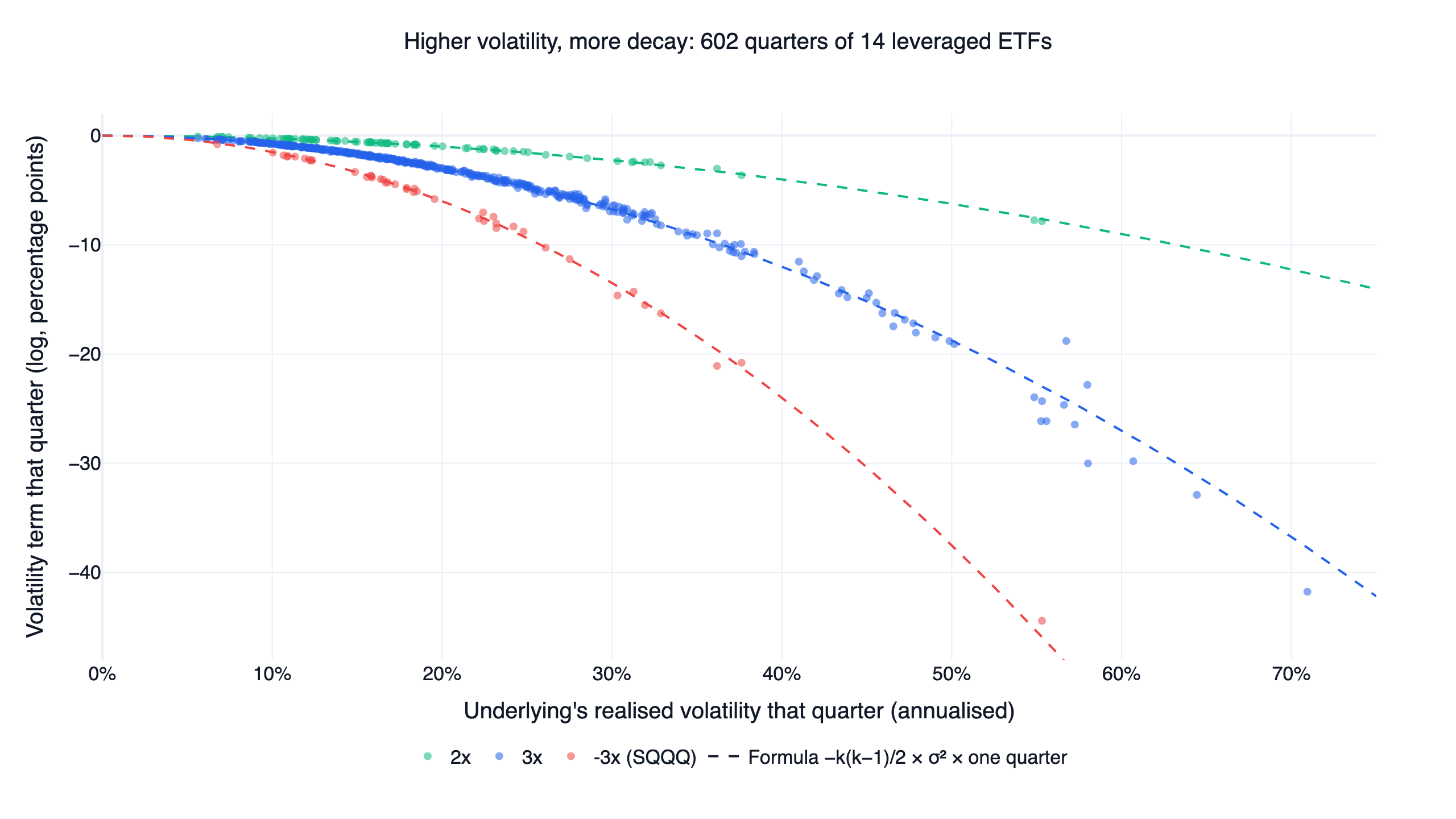
Each point is one fund in one quarter. The horizontal axis is the underlying's annualized realized volatility that quarter, the vertical axis is the quarter's volatility term, and each dashed line is the formula −k(k−1)/2 × σ² × one quarter. All three groups sit on their own line. Across 602 quarters the measured term and the formula differ by 0.13 points on average, and 95.7% of quarters are within 0.5 points. The largest miss is SOXL in the first quarter of 2020, at -41.8 points measured against -36.6 from the formula. The semiconductor index ran at 70.9% annualized volatility that quarter, and the higher-order terms the formula drops matter only on days with very large moves.
The factor k(k−1)/2 sets the speed. It is 1 for 2x, 3 for 3x and 6 for -3x. On the same QQQ, QLD's volatility term is -5.0 a year, TQQQ's -15.2 and SQQQ's -30.1, close to 1 : 3 : 6. The other input is the underlying's volatility. UPRO and SOXL are both 3x, yet UPRO loses 9.6 a year and SOXL 36.7, because SOXX's volatility (34.5%) is about twice SPY's (17.7%), and squaring makes that four times.
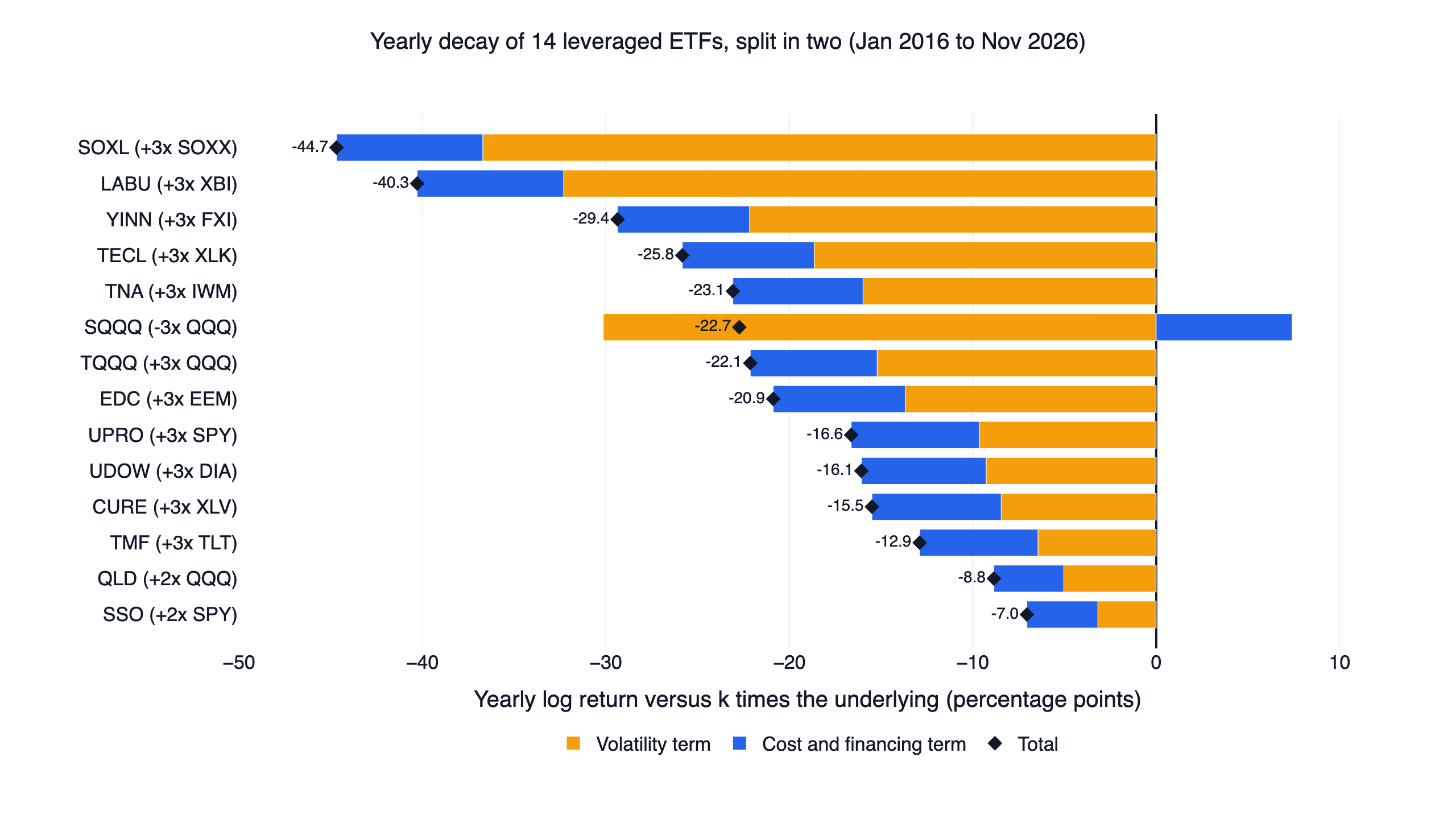
This chart draws the two terms from the key numbers table as bars, orange for volatility and blue for costs. The blue bars of the 3x funds are all about the same length, 6.4 to 8.0 points a year, so almost all of the difference between them is orange. SQQQ is the one fund whose blue bar points right, in its favour.
So two things decide how much a leveraged ETF decays: its leverage and its underlying's volatility. Volatility enters squared, so doubling it quadruples the decay.
Result 2: the cost term follows interest rates
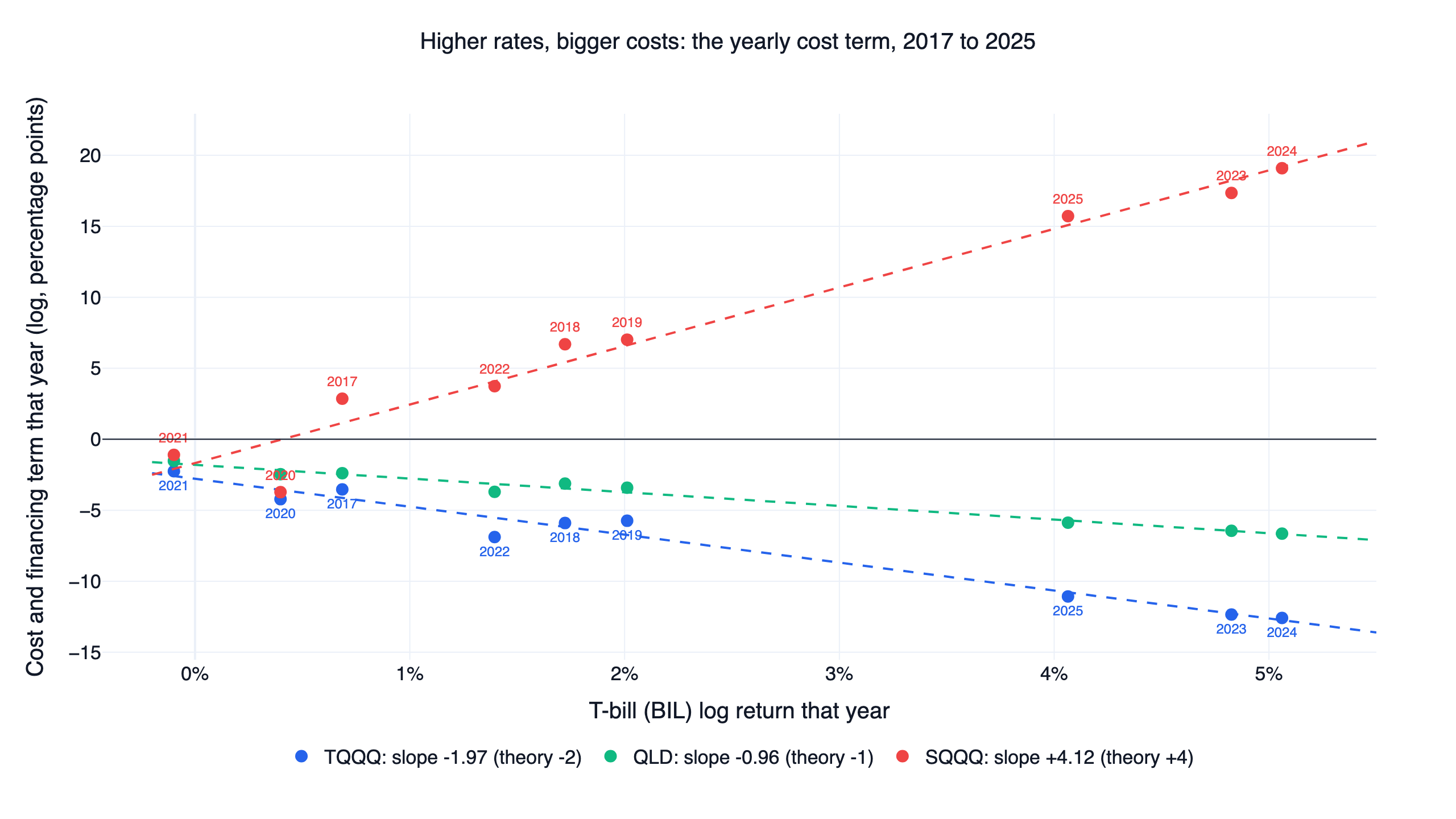
Each point is one full year. The horizontal axis is that year's log return on BIL, a Treasury bill ETF that stands in for short-term rates. TQQQ's cost term was -2.3 points in 2021, when rates were near zero, and -12.3 and -12.6 in 2023 and 2024, when they were near 5%. A regression over the nine years from 2017 to 2025 gives TQQQ a slope of -1.97 against a theoretical -2. Its intercept of -2.8% is what a year at zero rates would still cost. QLD's slope is -0.96 against a theoretical -1. The other 3x funds in the main table run from -1.67 to -2.67, and the two 2x funds are at -0.96 and -0.97.
SQQQ's slope is +4.12 against a theoretical +4. Higher rates push its cost term up: +17.4 points in 2023 and +19.1 in 2024. Its volatility factor is 6, though, so its volatility term averaged -30.1 a year. The interest it earns covers only a fraction of that, and SQQQ lost 99.97% from January 2016 to November 2026.
This matters for anyone extrapolating from old backtests. From 2016 to 2021, with low rates, TQQQ's cost term ran between -2.3 and -5.9 a year. From 2023 to 2025, with rates of 4% to 5%, it was worse than -11 every year, and 2026 to November 5 stands at -7.9. A backtest drawn mostly from the low-rate years understates what holding a leveraged ETF costs now.
Result 3: TQQQ year by year
| Year | QQQ | 3 × QQQ | QQQ cubed | TQQQ | Volatility term | Cost term | QQQ volatility |
|---|---|---|---|---|---|---|---|
| 2016 | 9.4% | 28.2% | 31.0% | 18.3% | -7.8 | -2.4 | 16.1% |
| 2017 | 32.7% | 98.0% | 133.5% | 118.1% | -3.3 | -3.5 | 10.3% |
| 2018 | -0.1% | -0.3% | -0.3% | -19.8% | -15.8 | -5.9 | 22.9% |
| 2019 | 39.0% | 116.9% | 168.3% | 133.9% | -8.0 | -5.7 | 16.2% |
| 2020 | 48.6% | 145.9% | 228.3% | 110.1% | -40.4 | -4.2 | 35.6% |
| 2021 | 27.4% | 82.3% | 106.9% | 83.0% | -10.0 | -2.3 | 18.2% |
| 2022 | -32.6% | -97.7% | -69.4% | -79.1% | -31.3 | -6.9 | 32.1% |
| 2023 | 54.9% | 164.6% | 271.3% | 198.3% | -9.6 | -12.3 | 17.9% |
| 2024 | 25.6% | 76.7% | 98.0% | 58.2% | -9.8 | -12.6 | 18.0% |
| 2025 | 20.8% | 62.3% | 76.1% | 34.4% | -16.0 | -11.1 | 23.6% |
| 2026 | 5.7% | 17.1% | 18.0% | -3.7% | -12.5 | -7.9 | 21.9% |
2016 starts at the close of January 4, and 2026 runs to November 5. The two terms are in log points.
- TQQQ beat 3 × QQQ in five years: 2017, 2019, 2021, 2022 and 2023. Those years had either low volatility (QQQ ran at 10.3% in 2017, for a volatility term of only -3.3) or a strong trend, so the compounding in the cube outweighed the decay. TQQQ's -79.1% in 2022 looks better than -97.7%, yet it is almost 10 points worse than the decay-free -69.4%.
- Volatile years decay most: in 2020 QQQ gained 48.6% at 35.6% volatility, the volatility term was -40.4, and TQQQ's 110.1% fell far short of 145.9%. In 2018 QQQ lost 0.1% and TQQQ lost 19.8%.
- Since 2023 the cost term has caught up: QQQ's volatility stayed below 24% from 2023 to 2025, for volatility terms of -9.6 to -16.0, while the cost term ran from -11.1 to -12.6. The two are now about the same size.
- 2026 to November 5: QQQ gained 5.7% and TQQQ lost 3.7%. On November 5 alone QQQ fell 6.5% and TQQQ 18.9%, and at the previous close TQQQ had still been up 18.8% for the year. Semiconductors were more extreme. SOXX rose 31.6% for the year at 51.3% volatility, SOXL fell 2.9%, and the volatility term alone was -70.5 points. On November 5 SOXX fell 12.1% and SOXL 38.7%, a day after SOXL had been up 58.5% for the year. The SOXL vs SOXX comparison shows the two side by side.
The decay sits in volatile days
We split every trading day from 2016-04-04 to 2026-11-05, the same days as the switch tests below, by QQQ's 20-day annualized volatility at the previous close. Days above 25% were 22.5% of the sample, about 2.4 years, and the rest made up about 8.2 years. Those 2.4 years carried 52.7% of TQQQ's volatility decay, with each day's volatility term computed as ln(1 + 3r) − 3 ln(1 + r) for QQQ's return r.
| Days | Share of days | QQQ log return per year | TQQQ log return per year | 3 × QQQ | QQQ daily Sharpe | TQQQ daily Sharpe |
|---|---|---|---|---|---|---|
| QQQ 20-day volatility ≤25% | 77.5% | 18.1% | 38.2% | 54.3% | 1.13 | 1.00 |
| QQQ 20-day volatility >25% | 22.5% | 15.1% | 2.1% | 45.3% | 0.61 | 0.53 |
On the volatile days QQQ still made 15.1% a year in log terms, and TQQQ made 2.1%. That table is the case for switching: hold QQQ when volatility is high and TQQQ when markets are calm, keep most of the leveraged return and skip more than half of the decay. Cooper (2010) built managed-volatility rules for leveraged ETFs on that idea. Volatility is easier to forecast than returns, so the rule cuts leverage when volatility rises. Moreira and Muir (2017) found that scaling equity exposure down after high variance raised the Sharpe ratio. The table above sorts days after the fact, though. The next section tests whether a signal known at the time captures the gain.
The volatility switch: four designs and how each had to pass
The rule has one line. At each close, compute the underlying's realized volatility over the past N trading days (standard deviation of daily returns × √252). Above the threshold, hold the underlying's 1x ETF. At or below it, hold the leveraged ETF. When the signal changes, trade at the next day's close. Cash is never held.
| Design | Leveraged ETF / fallback | Original setting | 9 neighbouring settings | Benchmark |
|---|---|---|---|---|
| TQQQ switch | TQQQ / QQQ | 20 days, 25% | 10/20/40 days × 20%/25%/30% | QQQ with dividends |
| QLD switch | QLD / QQQ | 20 days, 25% | same | QQQ with dividends |
| UPRO switch | UPRO / SPY | 20 days, 20% | 10/20/40 days × 15%/20%/25% | QQQ with dividends |
| SOXL switch | SOXL / SOXX | 20 days, 35% | 10/20/40 days × 30%/35%/40% | QQQ with dividends |
Each threshold sits near the index's long-run volatility: about 25% for the Nasdaq-100, 20% for the S&P 500 and 35% for the semiconductor index. The tests run from 2016-04-01, so that the 40-day volatility has data, to 2026-11-05. The rule, the settings and the pass conditions were fixed before any result was seen and were not changed afterwards.
"Beat" has one meaning here: a higher daily Sharpe ratio than buying and holding QQQ with dividends over the same dates, where daily Sharpe is the mean daily return ÷ its standard deviation × √252, with no risk-free rate. A design had to pass all five checks:
- Neighbouring settings: at least 7 of the 9 settings beat QQQ.
- Both halves: split at the midpoint (2021-07-20), the original setting beats QQQ in each half.
- Costs: finlab's default US fee and tax are both zero, so this check charges 0.1% on every buy and every sell for spread and slippage.
- A fixed mix with the same average weight: the TQQQ switch held TQQQ on 77% of days, so it had to beat 77% TQQQ plus 23% QQQ rebalanced monthly. This checks that the timing adds something beyond the average leverage.
- Without the best year: drop the strategy's best calendar year from both the strategy and QQQ, and the strategy still wins on the remaining days.
Volatility switch result: no design passed all five
| Design | CAGR | Daily Sharpe | Max drawdown | Settings beating QQQ | First / second half Sharpe | 0.1% per side | Fixed-mix Sharpe | Without best year | Result |
|---|---|---|---|---|---|---|---|---|---|
| TQQQ switch | 42.1% | 0.97 | -57.5% | 4 / 9 | 1.22 / 0.74 | 0.95 | 0.82 | 0.81 vs 0.76 | Failed (neighbours only) |
| QLD switch | 31.2% | 0.96 | -46.8% | 6 / 9 | 1.23 / 0.71 | 0.93 | 0.84 | 0.80 vs 0.76 | Failed (neighbours only) |
| UPRO switch | 28.4% | 0.86 | -46.1% | 0 / 9 | 1.14 / 0.60 | 0.83 | 0.74 | 0.75 vs 0.85 | Failed |
| SOXL switch | 60.1% | 1.02 | -72.5% | 5 / 9 | 1.168 / 0.86 | 0.99 | 0.84 | 0.92 vs 0.76 | Failed |
| QQQ with dividends | 19.1% | 0.90 | -35.1% | benchmark | 1.175 / 0.62 | — | — | — | benchmark |
| TQQQ buy and hold | 35.3% | 0.79 | -81.7% | reference | — | — | — | — | reference |
| QLD buy and hold | 29.7% | 0.81 | -63.7% | reference | — | — | — | — | reference |
| SOXL buy and hold | 35.5% | 0.82 | -90.5% | reference | — | — | — | — | reference |
All rows run from 2016-04-01 to 2026-11-05. "Without best year" is the strategy against QQQ. The best year was 2023 for the TQQQ, QLD and SOXL switches and 2021 for the UPRO switch.
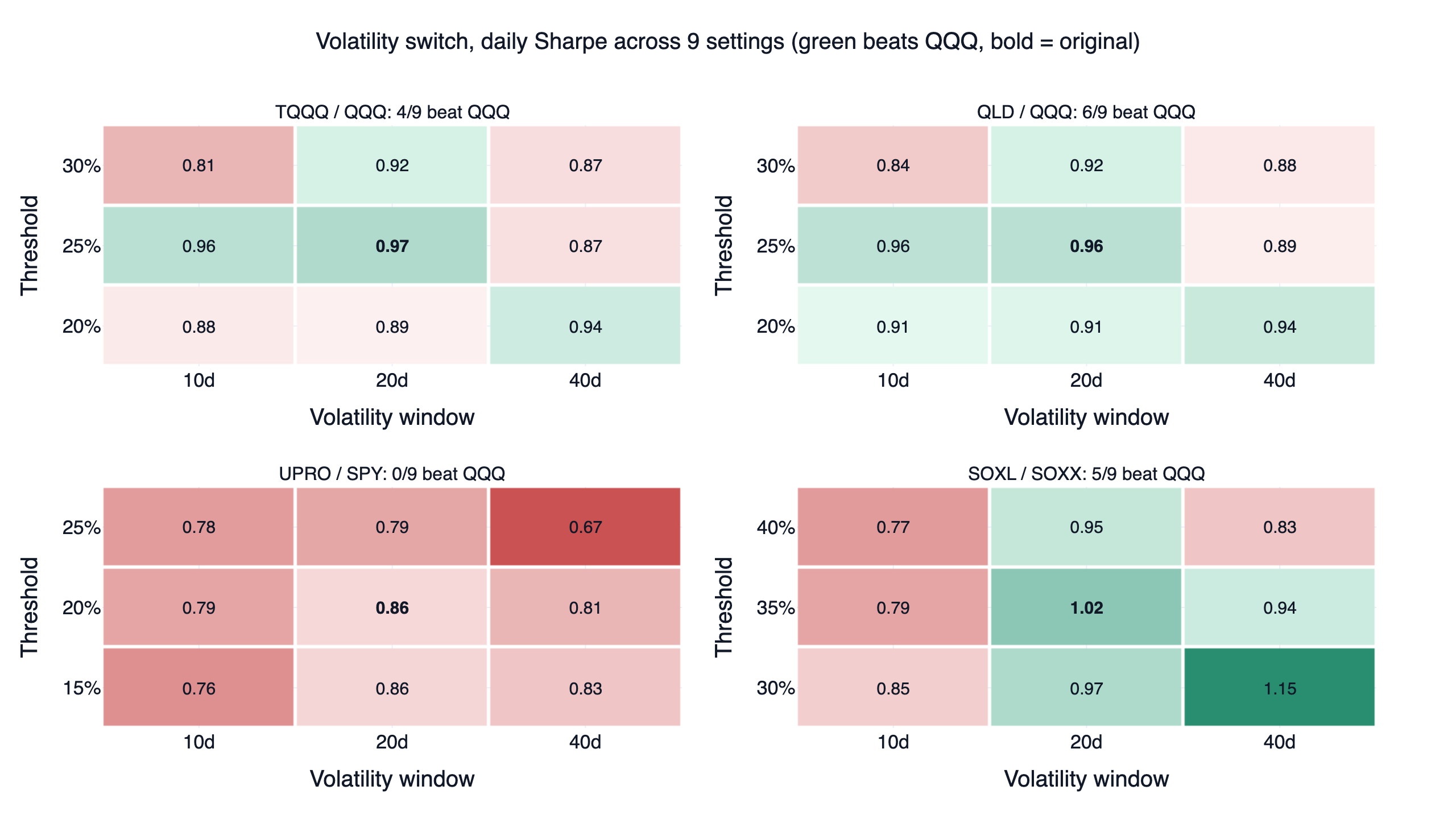
The TQQQ switch made the strongest case. It returned 42.1% a year, about 7 points more than holding TQQQ (35.3%). Its maximum drawdown was -57.5% against -81.7%, and its daily Sharpe of 0.97 beat QQQ's 0.90. It passed the halves, costs, fixed-mix and best-year checks. It failed the first: only 4 of its 9 neighbouring settings beat QQQ. The original 20 days at 25% scored 0.97. With the same 25% threshold, 40-day volatility scored 0.87, and 10 days at 30% scored 0.81. Five of the nine cells sit below QQQ's 0.90. The QLD switch had the same shape with 6 winners, one short of the 7 required.
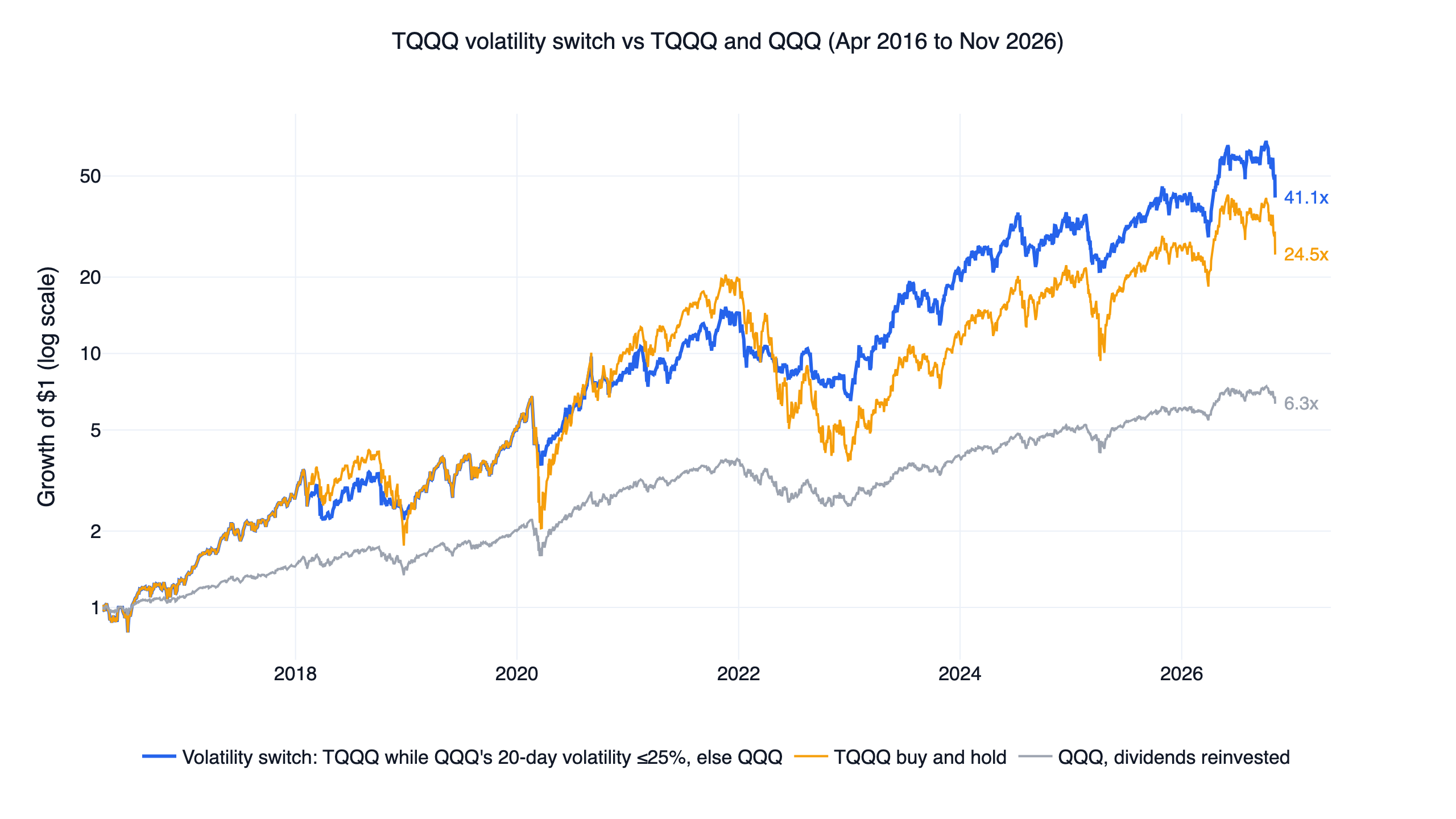
The interactive report below covers the TQQQ switch at its original setting, with every switch and the yearly returns:
Why it failed: volatile markets also hold the big rebounds
First, the timing is sensitive. The switch traded about 5.6 times a year (9.9 for SOXL), and each trade is a call that volatility is now high enough or calm enough. A 10-day window reacts to a single sharp drop and moves to QQQ too often. A 40-day window is slow to return to TQQQ after volatility fades. Five of the nine cells lose, so the result leans on the one setting that happened to be chosen.
Second, the most volatile days include the biggest rebounds. QQQ's 20-day volatility rose above 25% in late February 2020 and did not fall back below it until May 20. The switch held QQQ throughout and missed TQQQ's rally off the March low. In 2020 the switch gained 76.6% and TQQQ 110.1%. In 2022 it went the other way: the switch lost 51.6% and TQQQ 79.1%. The two kinds of year offset each other, and the average gain was small enough to vanish under a different setting.
Third, UPRO and SOXL fell short in different ways. All 9 UPRO settings lost to QQQ. SPY is calm, so with a 20% threshold the switch held UPRO on 82% of days. Avoiding part of the decay did not make up for the S&P 500's lower Sharpe ratio than QQQ's. The SOXL switch had the highest Sharpe of the four, 1.02, and gained 99.5% in 2026 while SOXL fell 2.9%. Its first half scored 1.168 against QQQ's 1.175, just short, and only 5 of 9 settings won. The UPRO vs SPXL comparison covers the two 3x S&P 500 funds.
Fourth, the fixed-mix check shows the timing helps, just not reliably. All four switches beat a fixed mix at the same average weight. The TQQQ switch scored 0.97, while 77% TQQQ plus 23% QQQ scored 0.82. Switching on volatility did avoid much of the decay. Its edge over plain QQQ was about 0.08, though, and that edge was not stable under these checks.
The code
The core is short. The snippet below splits TQQQ's yearly shortfall into the volatility and cost terms, then runs the TQQQ switch at its original setting. The full research.py covers the yearly and quarterly splits for all funds and the five checks for every switch design.
Show Code
import math

import finlab
import pandas as pd
from finlab import data
from finlab.backtest import sim

finlab.login()  # finlab walks you through sign-in when data is needed
data.set_market("us_fund")
close = data.get("us_fund_price:adj_close").loc[:"2026-11-05"]
qqq = close["QQQ"].dropna()    # market holidays are empty rows; drop them before taking returns
tqqq = close["TQQQ"].dropna()

# 1. Split each year into a volatility term and a cost term (log returns add up)
year_ends = qqq.groupby(qqq.index.year).tail(1).index
for start, end in zip(year_ends[:-1], year_ends[1:]):
    daily = qqq.loc[start:end].pct_change().dropna()
    qqq_log = math.log(qqq[end] / qqq[start])
    ideal_log = math.log((1 + 3 * daily).prod())   # daily 3x, no costs
    tqqq_log = math.log(tqqq[end] / tqqq[start])
    volatility_term = ideal_log - 3 * qqq_log
    cost_term = tqqq_log - ideal_log
    print(end.year, f"volatility {volatility_term:+.1%}", f"costs {cost_term:+.1%}")

# 2. Volatility switch: hold TQQQ while QQQ's 20-day volatility is at or below 25%, else QQQ
volatility = qqq.pct_change().rolling(20).std() * 252 ** 0.5
calm = (volatility <= 0.25).astype(float).loc["2016-04-01":]
position = pd.DataFrame({"TQQQ": calm, "QQQ": 1 - calm})
report = sim(position, trade_at_price="close", upload=False)

# 3. Compare daily Sharpe with QQQ with dividends on the same dates
curve = report.creturn.loc[:"2026-11-05"]
benchmark = qqq.reindex(curve.index).ffill()
for name, series in [("Volatility switch", curve), ("QQQ", benchmark)]:
    returns = series.pct_change().dropna()
    print(name, round(returns.mean() / returns.std() * 252 ** 0.5, 2))
In our environment this prints the two terms for 2017 to 2026, matching the yearly table (for 2023, volatility -9.6% and costs -12.3%), then 0.97 and 0.9.
Install the FinLab skill for your AI agent
You do not need to write this yourself. Install the FinLab skill in Claude Code, Codex or Gemini CLI with one command:
Show Code
npx skills add koreal6803/finlab-ai --skill finlab -g -yThen ask your agent in plain language, for example "split my leveraged ETF's yearly return into volatility decay and costs" or "rerun the volatility switch with QLD and a 30-day window, then run all five checks". Change one thing at a time and rerun the checks after each change. The agent setup page has the details for each tool, the AI-assisted setup walks through the first run, and FinLab Studio runs the same research in a browser.
Backtest method and limits
| Item | How it was handled |
|---|---|
| Window | The decay split runs from 2016-01-04 to 2026-11-05. 2016 starts at the close of January 4 and 2026 ends on November 5. The switch tests start on 2016-04-01. FinLab's US fund prices begin in January 2016, so 2008 is not covered |
| Universe | 15 leveraged ETFs and their 1x underlyings, plus BIL as the rate reference. Only the 14 funds whose daily returns correlate at least 0.99 with k times the underlying are in the main table. All 14 survived the decade, and leveraged ETFs that closed during it are not sampled, so the buy-and-hold comparisons with each underlying lean optimistic. The decay split itself is unaffected |
| Prices | us_fund_price:adj_close, dividend-adjusted closing prices rather than net asset values. Premiums and discounts to net asset value land in the cost term |
| Split method | Each calendar year and quarter is computed separately. The no-cost return chains k times the underlying's daily returns. The quarterly scatter uses only full quarters with at least 55 trading days |
| Look-ahead | The switch signal uses that day's close, and sim() trades at the next day's close. The volatile-day table sorts days by the previous close's volatility and describes where the decay fell. It is not a strategy |
| Costs | The main runs use finlab's US defaults, zero fee and zero tax. The cost check charges 0.1% per buy and per sell, which lowers daily Sharpe by 0.02 to 0.03 |
| Turnover | Each switch moves 100% of the portfolio from one fund to the other. The TQQQ and QLD switches trade 5.6 times a year, UPRO 5.2 and SOXL 9.9 |
| Taxes | None. Dividends are reinvested in full |
| Benchmark | QQQ with dividends, bought and held without sim() and without costs |
| Sample | Everything is in sample, with no out-of-sample period. The two halves are a stability check. Capacity is not estimated |
| Versions | Rerun on 2026-11-07 with finlab 2.3.8 and pandas 3.1.1, on prices through 2026-11-05 |
What this result does and does not say
In this setup and over these 10.8 years, leveraged ETF decay splits cleanly. The volatility term depends on the leverage and the underlying's volatility and follows the formula closely. The cost term depends on interest rates and has grown in the last three years. Both are the price of holding a leveraged ETF. Whether holding one beats its underlying over time depends on whether the underlying trends strongly enough and stays calm enough. QQQ trended strongly in this decade, and TQQQ's 34.0% a year still beat QQQ's 18.7%. Five other 3x funds with more volatile or weaker underlyings, TNA, EDC, LABU, YINN and TMF, trailed their own underlyings. LABU lost 85.9% and YINN 90.4% over the ten years.
Holding the 1x ETF when volatility is high did avoid part of the decay. All four switches beat a fixed mix at the same average weight, and the TQQQ switch cut the maximum drawdown by 24 points against holding TQQQ. What it did not show is a reliable edge over simply holding QQQ on a risk-adjusted basis. Under these checks, a different setting or a different half-decade could erase it. QQQ's 20-day volatility stayed above 25% for long stretches only four times, in late 2018, spring 2020, the first half of 2022 and spring 2025, which is a small sample.
For a volatility rule that passed its checks, the QQQ volatility targeting strategy sets QQQ's weight each month from its realized volatility and parks the rest in short Treasuries, without leverage, and has a strategy page updated daily. For leverage that passed, the US ETF rotation strategy and the US low volatility strategy both hold leveraged ETFs only while QQQ is above its 200-day moving average. A pure moving-average version is in the TQQQ 200-day moving average backtest, where seven rules also failed.
FAQ
Why do leveraged ETFs decay?
For two reasons. The first is the daily reset: the fund resets to 2x or 3x every day, so in a choppy market it keeps buying after rises and selling after falls. An index that gains 10% and then loses 10% leaves a 3x fund 6 points further behind. The second is fees and financing: a 3x fund borrows twice its assets and pays the short-term rate, a spread and a management fee. From 2016 to 2026 TQQQ trailed three times QQQ by 22.1 log points a year, 15.2 from volatility and 6.9 from costs.
How much does a leveraged ETF lose to decay each year?
It depends on the leverage, the underlying's volatility and interest rates. Among these 14 funds, the 2x SSO and QLD lost 7.0 and 8.8 points a year in total. The 3x UPRO lost 16.6, TQQQ 22.1 and SOXL, on the most volatile index, 44.7. Single years vary much more: TQQQ lost 6.8 points in 2017 and 44.6 in 2020.
How do you calculate volatility decay?
In log returns, the volatility term is about −k(k−1)/2 times the sum of squared daily returns, where k is the leverage. With annualized volatility σ held for T years, that is −k(k−1)/2 × σ² × T. At QQQ's 22.3% volatility, a 3x fund loses about 3 × 0.223² ≈ 15 points a year, in line with the measured 15.2. Across 602 quarters the formula missed the measured value by 0.13 points on average.
Is beta slippage the same as volatility decay?
Yes. Beta slippage, volatility decay and volatility drag all name the gap between a daily-reset leveraged fund and the leveraged long-run return of its index. This article's volatility term measures exactly that gap and keeps fees and financing in a separate cost term.
Do inverse ETFs decay faster?
Much faster. For -3x the factor is (-3)×(-4)/2 = 6, twice the 3 of a 3x fund. SQQQ's volatility term was -30.1 a year against TQQQ's -15.2. At high rates SQQQ's cost term turns positive (+19.1 in 2024), but that does not offset the volatility term, and SQQQ lost 99.97% from January 2016 to November 2026.
How do interest rates affect leveraged ETFs?
Higher rates raise the cost. TQQQ's cost term has a slope of -1.97 against the Treasury bill return, so each extra point of rates costs about 2 points a year. It was -2.3 in 2021 and -12.3 in 2023. The 2x funds have slopes near -1.
Why did TQQQ beat 3x QQQ in some years?
Because three times QQQ's simple return understates the decay-free return. A daily 3x fund with no decay would compound to QQQ's return cubed, so in years with a strong trend or low volatility the compounding outweighs the decay and TQQQ beats the simple 3x. That happened in 2017, 2019, 2021, 2022 and 2023. In every year, though, TQQQ trailed the cube.
Does switching to the unleveraged ETF in volatile markets work?
It reduced decay and drawdowns but did not reliably beat QQQ under these checks. The TQQQ switch returned 42.1% a year with a -57.5% maximum drawdown and a daily Sharpe of 0.97 against QQQ's 0.90, but only 4 of 9 neighbouring settings beat QQQ. The QLD switch had 6 and UPRO 0. Volatile markets often hold the sharpest rebounds, and the switch missed much of 2020's.
Further reading
- TQQQ 200-day moving average backtest: seven timing rules for leveraged ETFs and the three checks
- Ten US quant trading strategies: ten US strategies that trade through leveraged ETFs
- US breakout trend strategy and US academic factors backtest
- Fund page: TQQQ. More research on the blog
Reproduce it yourself
| File | Contents |
|---|---|
| research.py | Yearly and quarterly splits for every fund, plus all neighbouring settings and the five checks for each switch design. Name a design (for example python research.py tqqq_switch) to open its backtest report |
| data.csv | Daily equity of QQQ, TQQQ, QLD, SPY, UPRO, SOXX, SOXL, QQQ cubed, the no-cost daily 3x QQQ, 0050, 00631L and the switches, each starting at 1 |
| metrics.json | The statistics in this article, including the price checks, yearly and quarterly splits, rate regressions, the volatile-day split, and each switch's settings, checks, yearly returns and buy-and-hold comparison. Growth multiples and single-day moves come from data.csv |
| report_strategy_2026-11-07.html | The full interactive report for the TQQQ switch at its original setting |
The team behind this research is on the about page.
Disclaimer: this article is for education only and does not constitute investment advice. Past performance does not guarantee future results, and investing involves risk. Leveraged and inverse ETFs carry volatility decay and magnified losses, and a 3x fund can lose more than 80% within months. All results are in sample, and the two halves were not validated out of sample. The funds named are used to describe research results, not as recommendations.
Last updated: 2026-11 | Backtest window: 2016-01 to 2026-11 | Benchmark: QQQ with dividends | Author: FinLab Quant Research
FinLab AI
Want to build your own strategy?
Describe your stock-picking ideas in natural language. AI automatically validates, backtests, and gives you answers
Start Free